Select a table cell contents in Word 2007

Confession time. I had a picture in a table cell in Word and try as I might I couldn’t get the little black angled cursor to appear so I could select the cell’s contents. Frustrating – yep, I’d say so.

Nope – wrong arrow, the image is so close to the table cell it’s almost impossible to get the cell select arrow to appear.

 

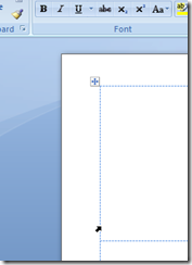
This is what it should  look like. 

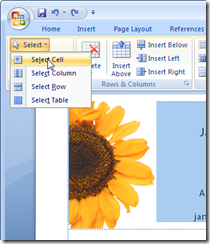
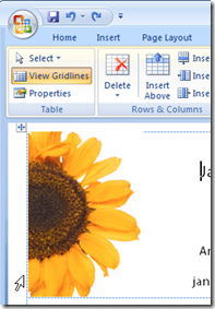
Then I remembered the new feature in Word 2007 – it’s on the Table Tools >Layout tab (so you have to have a table and click in it to see this option). On the far left is the Select button – new to Word 2007. Click it and you can select what to select. Oh! let’s back up a bit  here - it would be a good idea to click in the cell you want to select before you begin - forgot that bit.

Using this you can select a cell then right click and, as I did, choose Copy to copy its contents. Don't be fooled by the fact that not everything in the cell looks like it is selected - just trust that it is.

There are other options there that include Select Row, Select Column, Select Table – much easier than trying to juggle those little arrows when they just won’t appear.

Excel - trapping invalid data

There's a term that I love called GIGO - garbage in garbage out. When you're designing an Excle worksheet to solve a business problem you need to make sure that your data is correct or your worksheets won't give valid results.

Luckily, Excel's Data Validation tool helps you prevent incorrect data being added into your worksheet.

To set up a validation rule and to configure what will happen if incorrect data is entered, start by selecting the cells to which the rule should apply. Choose Data, Validation, Settings tab. Now, for example, to limit the data being entered to a whole number less than 200, select whole number from the Allow drop down list. When the Data area appears, choose Less Than and then in the Maximum area type 200.

To configure a user message to tell the user what is required, click the Input Message tab and type a title and a piece of explanatory text telling the user the limits to the type of Data you're expecting them to enter. This appears as a tooltip entry when any of the cells configured with the data validation rule is selected.

You can also specify what should happen if a user enters an incorrect value. To do this, click the Error Alert tab and select the type of indicator from the Style list. If the user enters incorrect data and if you have chosen the Stop style they will have two choices - Retry and Cancel and the invalid data cannot be entered into the cell. The Warning and Information styles both warn about the incorrect data but still allow it to be entered.

Once you've chosen the style, enter the Title and the Error Message which the user will see if the data in not correct. Click Ok and you can now test the rule.

Automatic Excel cell entries

We all love to save time and here's a great tip to make repetitive cell entries in Excel just so much easier to complete.

You do this by making a drop-down list in a cell so you can select your entry from it rather than having to type it fresh each time.

To do this:

1. Type the list of items to use in a single column in a spare sheet in the workbook.
   
2. Select these cells and choose Insert, Name, Define and type DataForList and click Ok.
   
3. Move to the sheet where the data goes, select the cells for the drop-down list and choose Data, Validation, Settings tab. From the Allow list choose List and, in the Source area, type =DataForList and click Ok.

Now, whenever you click a cell in this range you’ll see a list box indicator appear and you can choose the cell entry from the list.