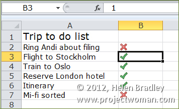
You can use Excel to fill a range with ticks and crosses to indicate Yes and No using a simple Excel Conditional Format.
To see this at work place a list such as to do items in column A of your worksheet. In column B, type the numbers 0 or 1 depending on when the task is completed or incomplete – 1 is completed, 0 is incomplete.
To make the numbers appear as checkmarks and crosses instead of 1 and 0, select the column of numbers and choose Conditional formatting from the Home tab on the Ribbon.
Select Icon Sets and then select the indicator set that has a checkmark, exclamation mark and cross in it.
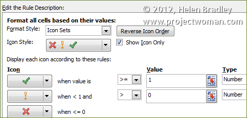
To fine tune this conditional formatting rule so it displays just the checkmark or the cross and not the numbers themselves and so it works correctly, keep the range selected and, from the Conditional Formatting dropdown list select Manage Rules. Select the Icon Set rule, select Edit Rule and click Format all cells based on their values in the top of the dialog.

Select the Show Icon Only checkbox and, set the checkmark to read >= 1 and set the Type to Number. For the ! icon set it to read > 0 and set its type to Number also. Click Ok.
You can change the icons by simply typing 1 or 0 into a cell.

