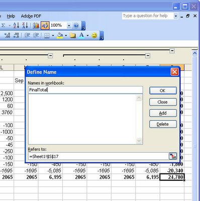
When you’re working with different areas on an Excel worksheet it sometimes helps to name the area or range as Excel calls it.
You might do this so that you can easily select a print area from a number of different printing areas on the worksheet or where you want to move very quickly to a named area which is in an out of the way place on the worksheet.
To name a range, select the cell or range of cells to name and choose Insert, Name, Define and give the cell or range a name. You can use whatever name you like, it just must be a single word name with no spaces and it can’t start with a number. When you’re done, click OK.
Now look up to the top left corner of the screen to the left of the formula bar you will see a small Name dropdown list. You can dropdown the list and select the named cell from the list and you will automatically go to it and, if it is a range, it will be automatically selected ready, for example, for printing.


Additional tips:
1. Alt-I-N-D still works as shortcut key (sequence) to popup the Names dialog.
2. You don’t need that dialog– you can just click&type in the worksheet. That mini-region at top-left which normally shows the cell you’re in (like A7, D13) and which may show a name if the cell/range you’ve selected is Named — well, just click in there and type whatever you want to Name this cell/range. When you press Return, it’s saved.
Advanced Tip:
Names have a “Scope”: they are either unique across the whole Workbook, or only unique within whichever Worksheet they’re defined on (in which case its name can be re-used/redefined on multiple Worksheets).
Or to look at it the other way up: if a name does not specify what Worksheet it refers to, it only refers to (is scoped to) this Worksheet ; else a name specifies what Worksheet it refers to, in which case it works exactly the same everywhere even on other Worksheets.
The idea is that data which varies per-Sheet can have per-Sheet names so that functions can be the same across those sheets yet still use Names.
Later Excel versions (eg v.2007) have a Scope dropdown on the Define Name dialog. Earlier versions (IIRC) let you edit the Refers To: field on that dialog to delete the sheetname specified to the left of the exclamation mark. ie, you’d just see “=!N18” or somesuch.
To refer to a Worksheet-Scoped Name from another worksheet, use the syntax “=!”, just the same way you’d type “=Sheet3!$A$9” for example.
To refer to Workbook-Scope Names, just type “=”.
Note that when you start typing a Name in a formula (eg, =MyNa…) :
1. you’ll see a dropdown in the edit-bar of available Name completions (press tab when on the one you want, same as for FunctionNames)
2. that list shows only the available Names HERE — ie, you’ll see all Workbook-Scope Names and all THIS worksheet’s Worksheet-Scope Names
whoops — the greater-than/less-than signs got swallowed as html.
The examples at end should read:
To refer to a Worksheet-scoped Name from another worksheet, use “=MYSHEET!MYNAME”.
To refer to a Worbook-scoped Name from another sheet, use “=MYNAME”
Example of how this is useful:
Say you have worksheets per year storing daily profit/loss. On each sheet you could have a worksheet-scoped Name covering the whole range of daily P&Ls, and a single Total cell on each sheet with “=sum(!DailyPnL).
At the start of each new year, just Copy a year’s worksheet, clear the data, and use it normally. You’ll still have a Total cell on it, working the way you’d expect
Neat trick #2:
If you then name each of these Total cells with a worksheet-scoped name, say “AnnualTotal”, you could have a single additional sheet at the start of your workbook with a single cell whose formula is “=sum(‘*’!AnnualTotal), adding up your total P&L To Date across all years.