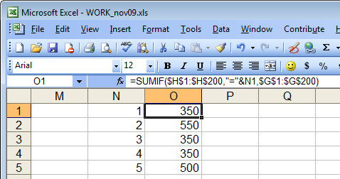
 I love SUMIF. It’s a handy tool for summarizing data. So, today I was checking how much I had invoiced a client – I have actual charges for stories I write in one column and the invoice numbers that these were charged under in another. I wanted a summary so I know the total of invoice 1 was $x and invoice 2 was $y.
SumIF is the tool to use. It goes like this:
=sumif(G1:G200,”=1″,H1:H200)
this sums the values in the range H1:H200 only if the corresponding values in the range G1:G200 is 1. So, it does the deed for Invoice #1. Repeat as required for invoices 2-20 – no way!
It is much easier if I place the numbers 1, 2, 3 and so on in cells of the worksheet and reference them in a single formula that can be copied rather than writing this 20 times… or 100 times… you get the picture… it’s simply not on to do this.
Problem is – how to refer to a cell in the SumIF function. This DOES NOT WORK! =sumif(G1:G200,”=N1″,H1:H200). Excel doesn’t see the N1 as a cell reference – it sees it as a value to match.
So, you have to write it differently:
=sumif($G$1:$G$200,”=”&N1,$H$1:$H$200
the “=”&N1 references the value in N1 as the one to match and the $ symbols are needed so the formula can be copied.

