Tuesday, March 19th, 2013

Excel – Sum a cell in all sheets but this one

Try this quick Excel formula to sum a cell in all the sheets except the current one

In Excel sometimes you’ll want to sum a cell value in all the sheets except the one that you’re currently working on. You might do this if you have a series of quarterly results that you want to add together to create a yearly total in the total sheet.

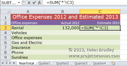
You can do this by typing the sheet name and cell for each cell to add but that would be very cumbersome. It will be a nuisance too if you try to select each cell in turn. Luckily Excel has a special feature that will help you do this. So, to sum all the values in, for example, cell C3 of every sheet in the current workbook except for the sheet you are currently working on, use this formula:

=SUM(‘*’!C3)

The ‘*’! part of the formula tells Excel that it should total all the sheets in the workbook except the current worksheet. When you press Enter Excel expands the formula so it will refer to the first and last sheets in the workbook. So, if you are summing that cell in a workbook that has sheets called YearTotal, Quarter1, Quarter2, Quarter3, and Quarter4 the formula will be expanded automatically so it reads:

=SUM(Quarter1:Quarter4!C3)

Be aware that if you add additional sheets to the workbook which appear inside the range of the sheets that are refered to in the formula then those additional worksheet cells will be included in the total.

If you don’t want this to be the case then make sure that any new sheets that you add appear outside the range of sheets that are included in the formula.

Helen Bradley

Wednesday, December 28th, 2011

Quickly access Excel 2010 formula requirements


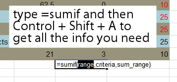
Ok.. so you want to use an Excel formula and you know it is, say, SUMIF that you want to use, but what data does it need and where?

Before you go searching through help or cranking up your browser, let Excel do the work for you. Just type =SUMIF in a cell and press Control + Shift + A and Excel will give you the list of data required. It’s dead simple and it saves heaps of time.


Helen Bradley

Thursday, July 22nd, 2010

Excel – cell reference in SumIF

I love SUMIF. It’s a handy tool for summarizing data. So, today I was checking how much I had invoiced a client – I have actual charges for stories I write in one column and the invoice numbers that these were charged under in another. I wanted a summary so I know the total of invoice 1 was $x and invoice 2 was $y.

SumIF is the tool to use. It goes like this:

=sumif(G1:G200,”=1″,H1:H200)

this sums the values in the range H1:H200 only if the corresponding values in the range G1:G200 is 1. So, it does the deed for Invoice #1. Repeat as required for invoices 2-20 – no way!

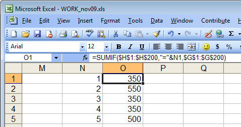
It is much easier if I place the numbers 1, 2, 3 and so on in cells of the worksheet and reference them in a single formula that can be copied rather than writing this 20 times… or 100 times… you get the picture… it’s simply not on to do this.

Problem is – how to refer to a cell in the SumIF function. This DOES NOT WORK!  =sumif(G1:G200,”=N1″,H1:H200). Excel doesn’t see the N1 as a cell reference – it sees it as a value to match.

So, you have to write it differently:

=sumif($G$1:$G$200,”=”&N1,$H$1:$H$200

the “=”&N1 references the value in N1 as the one to match and the $ symbols are needed so the formula can be copied.

Helen Bradley