Friday, October 23rd, 2009

Excel 2007 – Check for Duplicates


The new Excel 2007 has far superior tools for finding and removing duplicate entries in a list. Thankfully – because this has been a nightmare in earlier versions.

To find and remove duplicates from a list of data in Excel 2007 first format the area as a table by selecting it and, from the Home tab, choose Format as Table.

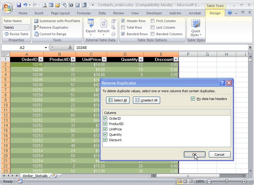
Click on any cell in the table and choose Table Tools > Design tab on the Ribbon.

Select Remove Duplicates to display the Remove Duplicates dialog. In this dialog are the Column headings for your data and all are selected by default. To remove the duplicate data from your worksheet leave all the column headings selected and click Ok.

If you want to remove rows where only certain data matches, leave the column headings for those particular rows selected and deselect the column headings for those columns which may have data that differs from one row to another. Now click Ok.

It is sensible to save your worksheet before running this Remove Duplicates option just in case you delete data by accident. If this happens and if you haven’t closed the file, you can recover it using the Undo button.

If you are using an earlier version of Excel, here are links to earlier relevant posts:
Excel – finding duplicates
http://www.projectwoman.com/2007/02/excel-finding-duplicates.html
Check for duplicates in an Excel list
http://www.projectwoman.com/2007/01/check-for-duplicates-in-excel-list-1.html

Helen Bradley

Wednesday, July 29th, 2009

Excel macro – Format By Contents

You can do so much with Excel macros – they can be so powerful.

Here is a macro that formats a cell depending on its contents when you type something in it.

If you type a number, or a formula that returns a number, it is formatted one way, if you type a date it is formatted another way and if you type a word it is formatted a different way.

The macro uses the OnEntry event which fires whenever something is entered into a cell. If you attach the macro to an Auto_Open macro you’ll ensure it is run whenever the workbook is opened.

To create the macro, choose Tools > Macro > Visual Basic Editor and, choose Insert > Module to add a module to the current worksheet. Type the code into the dialog.

Sub Auto_Open()
ActiveSheet.OnEntry = “formatCell”
End Sub

Sub formatCell()
If IsNumeric(ActiveCell) Then
ActiveCell.Font.Name = “Verdana”
ActiveCell.Font.Size = 12
ActiveCell.Font.ColorIndex = 46
ElseIf IsDate(ActiveCell) Then
ActiveCell.Font.Name = “Verdana”
ActiveCell.Font.Size = 10
ActiveCell.Font.ColorIndex = 50
Else
ActiveCell.Font.Name = “Times New Roman”
ActiveCell.Font.Size = 12
ActiveCell.Font.ColorIndex = 5
End If
End Sub

Sub Auto_Close()
ActiveSheet.OnEntry = “”
End Sub

Back in Excel choose Tools > Macro > Auto_Open to run the macro the first time to test it. Provided you have Excel configured to run macros, it will run automatically every time you open the workbook in future.

To learn more about Auto_open, AutoOpen and other fun macro naming conventions in VBA, visit this blog post:

What’s in a name? Auto_Open or AutoOpen What’s in a name? Auto_Open or AutoOpen
http://www.projectwoman.com/labels/Auto_Open.html

Helen Bradley

Tuesday, July 14th, 2009

Excel: Print a worksheet your way


When you need to print one version of a worksheet for yourself and another for the boss and you like it small and he likes it to be – well just how he likes it, then you need Views. The Excel Views tool lets you configure a worksheet for different printing options and to save these so you can use them again later on.

You can set views up so you do one for your boss and one for you. Or, you can set one up to print only the summary part of a worksheet and another to print the lot. Even if the print areas and the print settings change, Views let you preconfigure them so you don’t have to set them up manually every time. Better still, Views are saved with the worksheet so they’re always available.

Step 1
To save a set of printing settings, first set up your worksheet with the print settings you want to use including setting a print area if needed.

Step 2
To save this set up, choose View > Custom Views > Add (in Excel 2007 choose the View tab > Custom Views > Add). Type a name for the view that explains what settings you have selected. Enable the Print Settings checkbox and click Ok. You can now create another view and save it. Do this for as many different settings as you need. Save your worksheet.

Step 3
In future, before you print, choose View > Custom Views > select the View you want to use and click Show. Now go and print the worksheet – your settings were saved so you don’t need to configure them.

Helen Bradley

Thursday, July 9th, 2009

Excel page headers and footers


When you’re printing a 50 page worksheet, you want to hold onto the printed pages very carefully. If you don’t the entire project is prone to disaster as it is all too easy for the pages to get out of order and it’s nearly impossible to sort out the mess. So, either staple them very quickly or use the header and footer tool in Excel to add page numbers to all your pages.

Of course, while page numbers are one of the most common things you might put in a header or footer it isn’t the only thing. You can add everything from the date to your company’s logo.

To add a header or footer that will print on every page of an Excel workbook, choose View > Header and Footer in Excel 2003 or, in Excel 2007 choose Insert tab > Header & Footer. In Excel 2003 you can select from a range of preset headers and footers which are configured using typical combinations of items usually used in headers or footers – for example, sheet and worksheet names, page numbers, filename and folders.

If you’d prefer to create your own headers and footers, click the Custom Header or Custom Footer button and create your own design – this is the way you create a header or footer in Excel 2007 too.

Click in the Left, Center or Right areas of the dialog to place information at any of these places on the page. In Excel 2003 the buttons you can select from to add preset information aren’t labelled but you can usually tell what they are. From left to right, they let you change the font used, insert the page number, number of pages, date, time, filename and folder, filename, sheet name, and an image. In Excel 2007 they are labelled.

When adding an image to a header or a footer, make sure it is small enough to fit in the header area – there’s no tool in this dialog to resize the image if it’s too big. When you’re done, check the header by selecting Print Preview.

Helen Bradley

Wednesday, June 10th, 2009

Multi colored Excel charts


It isn’t always the case that you want to chart multiple series of data on a single chart. Sometimes you only have a single series and Excel, by default, plots all the bars or columns so they are colored identically. Boring!

Luckily, in Excel 2007 a solution is at hand. Simply select and right click the series and choose Format Data Series > Fill > Vary Colors by Point. Excel colors each bar a different color. Best of all, the colors are linked to themes so you can change the colors by changing the Theme – the theme tools are on the Page Layout tab.

So, no more boring single color charts – ever – please!

Helen Bradley

Monday, April 6th, 2009

Excel – calculating workdays with Networkdays


Excel has lots of very cool functions for doing all sorts of calculations. One of these is the NETWORKDAYS function.

You can use it to calculate the number of days between two dates taking into account holidays.

Start by placing the dates for the holidays in a range of cells across a row or down a column. Select this range and name it holidays using Insert > Name > Define.

The function calculates the number of workdays between two dates so place one, for now, in cell A1 and the other in A2. This function will calculate the days between the dates in cells A1 and A2 taking into account the holidays listed in the range called Holidays:

=NETWORKDAYS(A1,A2,Holidays)

If the NETWORKDAYS function returns an error make sure that you have the Analysis Toolpak installed as this function is stored in this toolpak. To install it in Excel 2003 choose Tools > Add-ins and enable its checkbox. In Excel 2007, click the Microsoft Office Button > Excel Options > Add-Ins and from the Manage list choose Excel Add-ins and click Go. In the Add-Ins Available list enable the Analysis ToolPak checkbox and click OK.

Helen Bradley

Tuesday, February 24th, 2009

Copy a worksheet – Excel 2007


I work with monthly worksheets and they develop over the month in such a way that I want the starting point for the next month to be where this month stops. So, I need to copy this month’s worksheet to make next month’s.

In Excel this is simple. Right click the tab at the foot of the worksheet and choose Move or Copy sheet. Make sure you click the Create a Copy checkbox so you make a copy or you’re toast – you’ll lose your original.

Now choose the position in the current workbook to make the copy or choose another or new workbook. Click OK and the copy is made.

I then strip out all of last month’s variable data and start over for this month… but I always make sure I made a copy before I do this, you never can be too sure.

Helen Bradley

Sunday, February 22nd, 2009

Excel 2007: quick format your data


I earlier versions of Excel there were some pretty horrid autoformats you could use to quickly format your tables. These are gone from Excel 2007 – thankfully!

Instead, Excel 2007 offers sophisticated formatting options, but they can be applied only if you’re prepared to convert your range to a table. However, this isn’t always a desirable outcome but luckily there is a work around.

Start by selecting your data and click Home tab > Format as Table and select a table format. You will notice that Excel applies an AutoFilter to your data which is typically the most obvious part of the conversion that you don’t want. Other things come with this table format too – if you have data alongside the table – but not part of it – and you delete a row from a table or insert a row into a table, the data alongside remains in place.

So, if you want to retain the nice formatting but not the table behaviour, click in the table and choose Table Tools > Design tab and click the Convert to Range option and click Yes when prompted to convert the table to a normal range. The range will go back to behaving like a typical Excel range and the formatting will be retained.

Helen Bradley

Monday, February 16th, 2009

Excel: Open multiple workbooks


If you’re like me, you will open Excel in the morning and then open a series of workbooks that you work on each day. You can save time in finding and loading these files by creating an Excel Workspace.

To do this, open all the workbooks you want to have opened each time you launch Excel and then save them as a Workspace file by choosing File > Save Workspace and type a name for the file. Click Save and you can then open all the workbooks at one time by opening the Workspace file. Of course, if you just want to open a single file you can open it as normal.

In Excel 2007 – find the Workspace feature by choosing View > Window > Save Workspace.

Another alternative for opening files automatically when Excel opens is to save the file to the XLStart folder – when you do this, the file is opened every time Excel launches.

Helen Bradley

Wednesday, December 17th, 2008

Fix the Headings in your Excel 2007 tables


Excel 2007 has some great tools for working with and formatting tables (previously called Lists in earlier versions). To create a table, select the range that contains the table data and from the Home tab select Format As Table. Select a table format style and, when prompted to, confirm that the selected area contains all the data for your table, whether or not your table has headers and click Ok. When you do this you will see that each heading cell displays a dropdown arrow to the right of its contents.

Unfortunately, if your headers are right aligned, the table headings will run into the arrows and be partially hidden. I don’t know why Microsoft doesn’t create a fix for this because it looks awful. To avoid this happening, select the heading cells, right click and choose Format Cells. Click the Custom setting and type @ and four spaces and click Ok. This should add sufficient spaces to the right of a heading to move the headings a little to the left so the headings can be seen clearly. Now it all looks much nicer as you see above.

Helen Bradley

Page 2 of 512345