Tuesday, September 18th, 2012

Trevor’s Quick Excel Tip – Navigate cells

Move around the cells in your workbook without touching your mouse using the Up and Down and Left and Right Arrow keys. To jump to the edge of the current block of data press Ctrl + the appropriate arrow key – so to move to the last row press Ctrl + Down Arrow.

Helen Bradley

Tuesday, February 22nd, 2011

Excel – copy a chart or worksheet as a picture

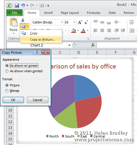
Image showing how to copy part of a worksheet or a chart as a picture

Sometimes you need to place a copy of a worksheet or a picture of an Excel chart onto your website or into a document. When you need only the image itself (not the link or an embedded version of the worksheet) you can make a copy of the area or graph as a picture.

So, with the worksheet open, select over the area that you want to convert to a picture. Or, if you need a picture of a chart select the chart. Now, from the Home tab, click the Copy dropdown list and choose Copy As Picture.

From the dialog which appears, choose Bitmap if you want an image the same size as you see it on the screen. To get an image you can make larger than this, choose Picture as this creates an image which scales well.

Then select either ‘As shown on screen’ or ‘As shown when printed’ as required. Click Ok and the picture will be copied to the Windows Clipboard. You can now paste the image into another application using that application’s Paste tool.

Helen Bradley
Thursday, February 17th, 2011

Excel – Hide a sheet in a workbook

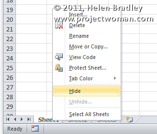
Excel hide a sheet in a workbook from view

If you have data on a worksheet that you don’t want others to see, you can hide the sheet but in such a way that the data on that sheet can still be used in formulas, for example.

To do this, right click the sheet tab for the sheet to hide and select Hide.

Now that the sheet is hidden, you can unhide it if necessary at a later date by right clicking any sheet’s tab and choose Unhide and then select the sheet to unhide.

If you hide the last sheet in the workbook, it will be less obvious to a user that there is a hidden sheet that they’re not being given access to.

Helen Bradley

Friday, February 11th, 2011

Excel 2007 & 2010 – Hidden add-ins

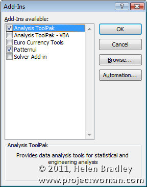
Excel 2007 2010 analysis toolpak lookup wizard solver add-in

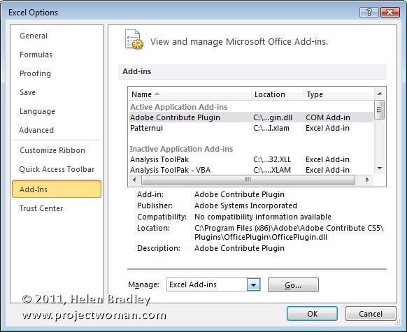
Excel 2007 & 2010 come with a number of add-ins that you can get to by choosing the Options button (File in Excel 2010) and choose Excel Options (Options in Excel 2010) and click Add-ins. From the Manage dropdown list choose Excel Add-ins and click Go.

Image explaining how to install the Excel 2007 2010 analysis toolpak lookup wizard solver add-in

A list of available Add-ins appears in the list. Any that don’t have their checkboxes checked aren’t enabled right now.

One you might want to enable is the Analysis Toolpak – this gives you access to functions like RANDBETWEEN and NETWORKDAYS. There’s also possibly a Lookup Wizard (in Excel 2007 only – it was discontinued in Excel 2010) and a Solver add-in in the list.

Click on any of the Add-ins to add them to Excel. Once you do, they’ll be available every time you launch Excel.

RANDBETWEEN is a handy function for filling cells with a random value. It’s syntax is RANDBETWEEN(startvalue, endvalue) so to fill a range with values between 100 and 200 use =RANDBETWEEN(100,200) then copy it to the range to fill. You can read more about the function here: Random numbers in Excel.

NETWORKDAYS  will calculate the number of working days between two dates. You can read more about this function here: Excel – calculating workdays with Networkdays.

Helen Bradley

Page 3 of 3123