Sunday, December 1st, 2013

Google Kills Spreadsheet Gadgets

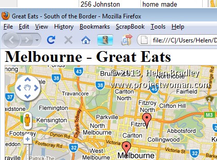
This is the old map gadget from Google – it doesn’t exist any more and the maps created using it won’t exist soon either.

If you’re asking yourself: What happened to Google Docs Gadgets? – the answer isn’t anything you want to hear

I loved Google Drive (formerly Google Docs) gadgets. These were advanced options you could use with Google spreadsheets.

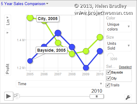
There was a Motion Chart gadget which helped you to create a great looking motion chart. You could set it up the way you wanted it to look and save those settings to the defaults. Click Publish and you’d get the code for the chart and you could embed it into a blog or website. Now it’s gone and the alternative is pretty awful by comparison. You can’t preset the motion chart settings – well you can try – but they aren’t saved with the worksheet and you can’t configure it and then put it on your website or blog. The chart keeps reverting to the default settings making it a whole lot less useful than it used to be.

 This and other old Gadgets either don’t exist in Google Drive or they have a really reduced functionality. 

Don’t get me started on the Map Gadget

Please don’t ask me about this one. This is so totally totally sad! The map gadget let you type a series of addresses into a Google Drive spreadsheet and you could select them and add the map gadget and it would plot the locations on a map.

It was A W E S O M E. And you know what? Google killed it – D E A D.

There is no map gadget – not even one which works horribly(like the other charts that replace deprecated gadgets) – it’s all gone. The only saving grace is that some folks have created apps to fill the gap and MapAList.com does a good job of taking the data from a Google Drive spreadsheet and plotting it on a map. Only I wish I didn’t have to use it – the old Google Gadget was a heap easier to use. To help you get started with MapAList I created a Youtube video that goes through the process.

This is why I hate the cloud

Yep.. there are things I hate about the cloud. Before the cloud took over our lives we bought software and it worked. If a developer made a new version of the software with new features – of if they removed old ones, we  could decide to upgrade or not.

The  cloud changed all that. Now Google makes changes and not only can we not do what we want to do but things we made don’t work anymore. The map gadget is being deprecated – for that read folks who used it in the past will find their published maps won’t work in the future. Don’t you hate that?

So what other bad news is there?

Sadly there is a lot. Google not only killed gadgets but it made a half hearted attempt at mollifying us with some new charts. Problem is that they suck – really, in contrast to what we had, they are pretty awful. They don’t have headings – so you can’t add a heading to charts like the motion chart, table chart, organization chart etc.  So, if you post a chart to your blog you’ll have to find another way to title it – really! Table charts used to be able to filter data – now they can’t – the list goes on.
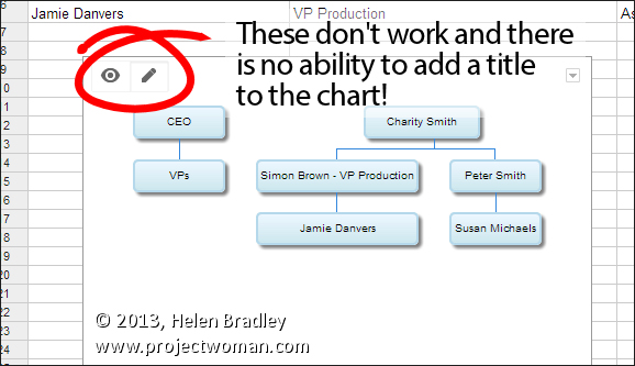

This is the new Organization chart – it is horrible, no title, buttons that don’t work and limited customization options – Shame Google Shame!

So, what can you do?

Bellyache about them – like I am.

Realize that all those blog posts out there that talk about Google Docs Gadgets are now wildly out of date – they are mostly useless as the charts don’t work like they use to.

Learn JavaScript – Google has a developer tool that you can use to make charts for web pages – but it is all done using JavaScript and the instructions and the examples on the Google site lack any real detail so, unless you really know what you are doing – they are hard to follow. Expect to put in a lot of trial and error to get it all working – and, to add insult to injury, you have to test your code online – the scripts won’t work on a local machine.

Hope someone creates better solutions. The folks at MapAList.com have done a good job of simplifying map creation. Hopefully other developers will create solutions that give us the functionality that Google saw fit to remove.

Stop talking about the cloud as being the panacea of all ills – it too often sucks and it disadvantages users when companies like Google take away functionality from their products.

OK.. rant over..


… for now  😉


Helen Bradley

Friday, November 15th, 2013

Google Drive Spreadsheet Notifications

Google Drive’s spreadsheets are liable to be shared and edited by many people.

This can potentially compromise the integrity of their data, so it’s a good idea to keep track of the changes made. Fortunately, Google provides a notifications service so the spreadsheet’s owner can do just that.

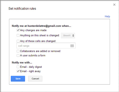
To access the notification rules, open the spreadsheet you want to track and select Tools > Notification Rules…. The resulting dialogue allows you to choose what changes to track. If only some data is critical, you can choose to only track a specific sheet or cell range. If you’ve set up a form to feed its result into your spreadsheet, you can choose to be notified whenever somebody submits the form. Choosing email – daily digest will add the notification to a daily email that contains all of your notifications that have this rule selected. Email right away immediately sends the specific notification to you.

Click Save when you are done. Your new notification rule will be the first on a list of all the notification rules for that spreadsheet. From the list you can add new rules, or edit or delete an existing one.

Helen Bradley

Friday, March 15th, 2013

Motion charts in Google Docs

Gadgets allow you to do things with Google Docs that would be time consuming if not beyond most people’s skills to create in a program like Excel. In this article I’ll demonstrate how to create a motion chart in Google Docs spreadsheet.

Prepare the data
In the first column of a new worksheet type the name of the item you’re charting such as office locations – we’ll use City and Bayside. In the next column, type the period that the data is for – this needs to be a time field such as year, week or quarter. The data needs to conform to ISO8601 so use 2011 for a year, 2011W08 to enter week eight of 2011 or 2011Q2 for second quarter 2011.

In the next column, type the data to plot such as Profit. The next columns are optional but we’ll add one which records units sold. To have some data to work with, add at least five years of data for the two offices.

Add the Gadget
Select over the entire range (including headings), and choose Insert > Gadget > Charts and scroll to find the Motion Chart and click Add to Spreadsheet. In the dialog which appears, the range should already cover the selected range, leave the Default State empty for now and type a title for your chart such as 5 Year Office Comparison and click Apply & Close.

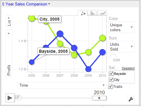
The chart appears on the screen but requires some customisation to  work. From the fly out menu of Y axis options on the left select Profit and then from the X axis dropdown list select Time so you plot Profit against Time.

From the Color dropdown list, select Unique Colors and from the Size dropdown list, select Units Sold.

Click the Play button and the chart will play showing the change in your data over time. The Y axis movement shows movement in Profit and the size of the bubble shows change in Units Sold.

The tabs change the chart from a Bubble to a Column or Line (this is not a motion chart).

If you click the office checkboxes and Trails you will see additional labels on your data and to the right of the Play button is a slider which controls playback speed.

Save the default
Wind the play button back to the beginning. Click the Settings button and click Advanced and Advanced again. Double click the state string to select it, right click and choose Copy. Click the chart title to display the chart menu, click Edit Gadget and paste the string into the Default State textbox. Save the worksheet and the chart will appear whenever the worksheet is viewed and it will be configured as you set it up to look.


Helen Bradley

Thursday, February 21st, 2013

Google Docs: Data Validation

Google Docs has the ability to use data validation to automate and manage data entry into cells in a spreadsheet. One way to do this is to limit the data that can be entered into a cell to a selection from a list that you create.

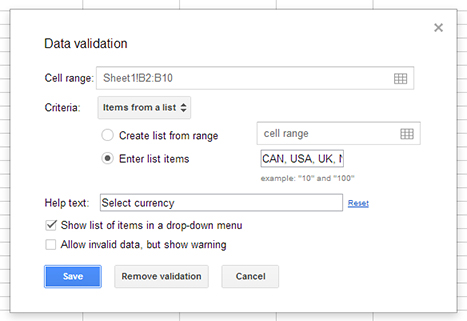
To see this at work, open an existing spreadsheet or create a new one. Select the cells into which the data will go and choose Data > Validation. From the Criteria dropdown list, select Items From a List and then click Enter List Items. Type each item for your list into the box separating entries from each other with a comma. Make sure the “Show list of items in a drop-down menu” is checked and if you don’t want a user to select anything that’s not in the list, then disable the “Allow invalid data, but show warning” checkbox. Click Save to save the validation options.


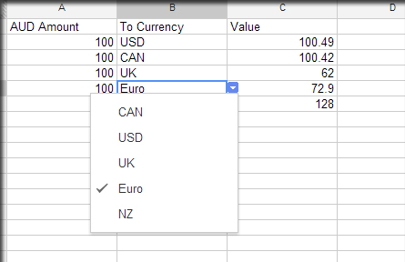
Now, when you enter data into any of the cells in the range you have configured this data validation rule for, you will see a dropdown indicator appear to the right of the cell. Click this and you can select an item from the list that is displayed below the cell. This data is entered into the cell in the same way as any data would be entered so you can, for example, use it in calculations by referring to the cell contents. In the example worksheet shown, a formula is used the cells in column C to calculate the converted value by checking what currency has been chosen and then multiplying the value in column A by the appropriate conversion rate.

It’s also possible to use other validation options using the Data Validation dialog. You can limit a cell entry to a number which meets certain criteria or to a text entry that contains or does not contain certain text or which is a valid email address or URL. You can also require that a date is entered within a certain range of dates or before or after another date.

You can force a user to comply with the data validation rules that you have created or allow them to enter an “invalid” value but warn them that they are about to enter data that doesn’t comply with the rule.

These data validation tools available in Google Docs are similar to those that you’ll find in other spreadsheet applications such as Excel.

Helen Bradley

Tuesday, November 6th, 2012

Trevor’s Quick Excel Tip – Select Everything

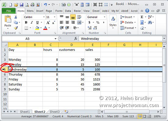
To select an entire row or column in an Excel worksheet, click the column letter or the row number. To select multiple columns or multiple rows click and drag over the column letters or row numbers to select. To select the entire worksheet, click the empty box at the intersection of the Rows and Columns in the top left of the worksheet.

Helen Bradley

Thursday, October 18th, 2012

Holiday Gift Budget Worksheet

Don’t blow the budget this holiday season!

Our holiday gift buying budget worksheet will help you avoid a Yule tide spending blow out.

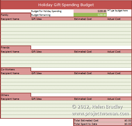
In the interests of helping you better control your spending this Holiday Season we have a free spreadsheet download in the form of a Holiday Gift Spending Budget.

Grab this version for Excel 2007/2010/2013 – gotta love the formatting available in those versions.

If you’re stuck in the land of Excel 2003 and earlier (or want to use it in Zoho, Google Docs, OpenOffice.org or anything else that can read Excel files), then grab this plainer but still fully functional version.

The worksheets are protected against wiping out key formulas and entering data in the wrong cells but there’s no password there so you can easily unprotect if you desire.

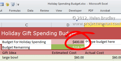
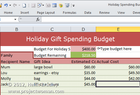
To use this worksheet, download the one for your Excel version, open it in Excel (or another compatible program), and then, in cell D2 type the amount you can afford  to spend.

Then add entries for family, friends, co-workers and others – determine what you will get them and  how much you are budgeting to spend. At this stage you can see if you are on track or already over budget.

As you buy presents, fill in the actual amount spent and in cell D3 you will see what you still have to spend of your budget amount or if have spent all you have allowed for.


Helen Bradley