Thursday, April 11th, 2013

Drawing Attention with a Drop Cap
One easy and fun way to add visual interest to a text heavy page is to use a Drop Cap. A Drop Cap is when the first letter of a paragraph is increased in size and, more often than not, put in a more ornate font.

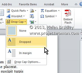
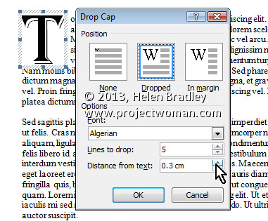
To create a Drop Cap, place your insertion point in the paragraph you wish to start with a Drop Cap. Then, choose Insert on the Ribbon, click Drop Cap > Drop Cap Options. The ‘Drop Cap Options’ allows you to either insert the Drop Cap into the paragraph, with ‘Dropped’, or place it separate from the text, with ‘In margin’. If you’re unsure what to use, I would suggest ‘Dropped’ and increase the ‘Distance from text’ setting to .3cm and the ‘Lines to drop’ setting (which affects the Font size of the actual Drop Cap) to 5 and click OK.

To change the font of the Drop Cap, you can either select the font you want directly in the ‘Drop Cap Options’ window or highlight the letter (which appears in a Frame) afterwards and changing it. You could even use Format, Borders and Shading, Shading tab to fill the frame with colour.
Helen Bradley
Labels: 2010, 2013, big, Cap, Distance from text, drop, Drop Cap, first, format, letter, Lines to drop, Microsoft Office, Microsoft Word, Office, tip, Word
Categories:office
posted by Helen Bradley @ 6:30 amNo Comments links to this post
Saturday, April 6th, 2013

You need to set up PowerPoint 2013 so it can find and save your templates.
I encountered a problem recently with PowerPoint 2013 not being able to save templates to the correct location much less find my new templates once I had created them.
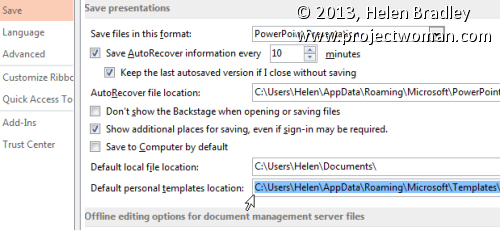
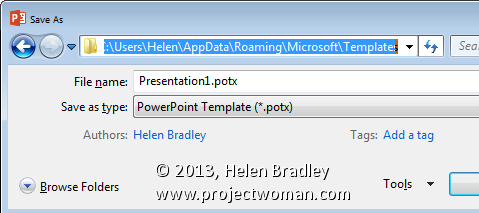
The problem appears to be with the PowerPoint 2013 setup so first go to PowerPoint and choose File > Options > Save and make sure that you have your Default Personal Templates location set up in this box. For me it is c:\Users\Helen\AppData\Roaming\Microsoft\Templates\. You will replace Helen with your own <user name>.

Once you set up this location, in future when you go to save a file as a template you will choose File > Save As, click Computer and then click Browse. From the Save As Type drop down list, select PowerPoint Template (*.potx) as the type of file to save and type a name for your template.

PowerPoint will automatically go to the folder that set as your Default Personal Templates location so all you need to do now is to click Save and save your template.
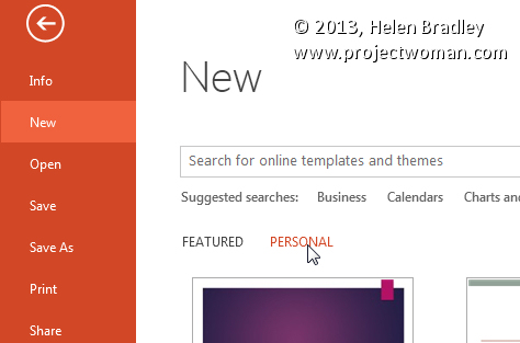
In future when you choose File > New you will see that both FEATURED and PERSONAL options appear below the Search box. Click PERSONAL as that is where you will find the templates that you created and saved. If you had personal templates stored for use in PowerPoint 2010 these will be in this same location.
Unfortunately Office 2013 doesn’t make it clear where templates are stored or how you can get to your own templates so hopefully this will help you in PowerPoint.
I haven’t had the same difficulties with Microsoft Word 2013 but then my Default Personal Templates location was already set up in Word 2013. If you have trouble finding your Word templates then I suggest you try the same process as shown here for PowerPoint but do it in Word 2013. Set up your Default Personal Templates location in Word – in this case my folder is c:\Users\Helen\AppData\Roaming\Microsoft\Templates\Custom Word Templates\.
Helen Bradley
Labels: configure, default personal templates location, options, PowerPoint 2013, save a template, save as type, template folder
Categories:office
posted by Helen Bradley @ 8:31 am2 Comments links to this post
Sunday, March 31st, 2013

Create a button in Excel to move the user to another worksheet
It is easy in Excel to create a button on a worksheet that you can click to go to another sheet in the workbook. It is also a fun way to get started with macros in Excel if you have never made one before.
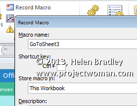
To do this, first decide which sheet will contain the button and which sheet you will select when you click, the button. We’ll add a button to sheet1 to take us to sheet3. So, click in Sheet 1 and, from the Developer tab on the Ribbon, choose Record Macro. If the Developer tab is not visible click here to find out how to display it.
Type the Name GoToSheet3 (a macro name must be all one word) and from the Store Macro in List choose to store the macro in This Workbook and click Ok.

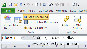
Click the tab for Sheet 3 and then click Stop Recording on the Developer tab. The macro will be recorded and stored automatically for you.

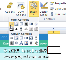
To add a button to Sheet 1 that will run the macro, first return to Sheet 1 and from the Developer tab on the Ribbon select the Insert option and click the Button (Form Control) option at the top of the drop down list. You must choose the Form Controls and not the Active X Controls.

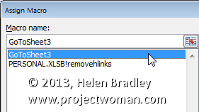
Drag a button onto the worksheet and when the Assign Macro dialog appears, click the GoToSheet3 macro and click Ok.

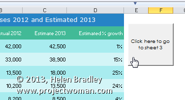
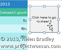
Select the text on the button and type Click to go to Sheet 3.

Click outside the button to unselect it and then click on the button to see it at work. When you click it you will be taken automatically to sheet 3.
If you need to make changes to the text on the button right-click on it to get access to the text. You can’t click it to select it because clicking it runs the macro attached to it.
Helen Bradley
Labels: assign macro, Excel, Form control, record maco, run macro from a button
Categories:office
posted by Helen Bradley @ 1:20 pm7 Comments links to this post
Monday, March 25th, 2013

When Excel won’t total a PivotTable there is a reason why – and a workaround
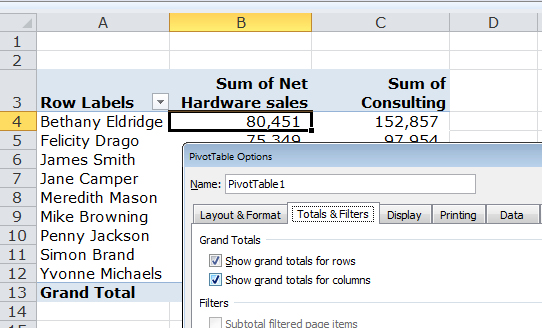
When you are working with a PivotTable in Excel and if the data you are looking at comes from two different columns in the original worksheet you won’t be able to create automatic totals for it in the PivotTable.
So, as much as you ask Excel for totals, you’ll be disappointed.

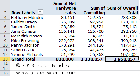
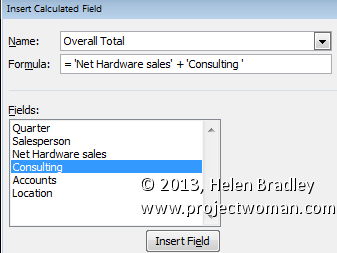
However, you can create manual totals. To do this, click in the table and from the Options tab choose Fields, Items & Sets > Calculated Field. In the dialog, click in the Name box and type the name Overall Total. Click in the Formula box and write a formula that totals the fields you want to total. In our example it will be Net Hardware Sales plus Consulting.
To write the formula click next to the = symbol in the Formula box. Click Net Hardware Sales in the Fields box and click Insert Field. Add a + symbol to the formula, then click Consulting in the Fields box and click Insert Field.
The resulting formula will read: = ‘Net Hardware sales’ + ‘Consulting ‘
When you are done, click Ok and the calculated field will be added to the table and it will be visible alongside the other fields in the PivotTable.

Helen Bradley
Labels: create custom calculated fields, create custom totals, Excel, manual totals, pivot table, pivottable
Categories:office
posted by Helen Bradley @ 11:12 amNo Comments links to this post
Tuesday, March 19th, 2013

Try this quick Excel formula to sum a cell in all the sheets except the current one
In Excel sometimes you’ll want to sum a cell value in all the sheets except the one that you’re currently working on. You might do this if you have a series of quarterly results that you want to add together to create a yearly total in the total sheet.
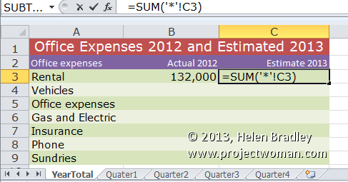
You can do this by typing the sheet name and cell for each cell to add but that would be very cumbersome. It will be a nuisance too if you try to select each cell in turn. Luckily Excel has a special feature that will help you do this. So, to sum all the values in, for example, cell C3 of every sheet in the current workbook except for the sheet you are currently working on, use this formula:
=SUM(‘*’!C3)
The ‘*’! part of the formula tells Excel that it should total all the sheets in the workbook except the current worksheet. When you press Enter Excel expands the formula so it will refer to the first and last sheets in the workbook. So, if you are summing that cell in a workbook that has sheets called YearTotal, Quarter1, Quarter2, Quarter3, and Quarter4 the formula will be expanded automatically so it reads:
=SUM(Quarter1:Quarter4!C3)
Be aware that if you add additional sheets to the workbook which appear inside the range of the sheets that are refered to in the formula then those additional worksheet cells will be included in the total.
If you don’t want this to be the case then make sure that any new sheets that you add appear outside the range of sheets that are included in the formula.
Helen Bradley
Labels: all sheets, automatic sum, Excel, formula, sum
Categories:office
posted by Helen Bradley @ 9:49 am2 Comments links to this post
Friday, March 15th, 2013
Gadgets allow you to do things with Google Docs that would be time consuming if not beyond most people’s skills to create in a program like Excel. In this article I’ll demonstrate how to create a motion chart in Google Docs spreadsheet.

Prepare the data
In the first column of a new worksheet type the name of the item you’re charting such as office locations – we’ll use City and Bayside. In the next column, type the period that the data is for – this needs to be a time field such as year, week or quarter. The data needs to conform to ISO8601 so use 2011 for a year, 2011W08 to enter week eight of 2011 or 2011Q2 for second quarter 2011.
In the next column, type the data to plot such as Profit. The next columns are optional but we’ll add one which records units sold. To have some data to work with, add at least five years of data for the two offices.
Add the Gadget
Select over the entire range (including headings), and choose Insert > Gadget > Charts and scroll to find the Motion Chart and click Add to Spreadsheet. In the dialog which appears, the range should already cover the selected range, leave the Default State empty for now and type a title for your chart such as 5 Year Office Comparison and click Apply & Close.
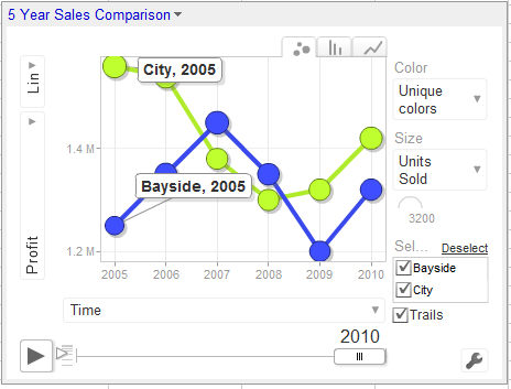
The chart appears on the screen but requires some customisation to work. From the fly out menu of Y axis options on the left select Profit and then from the X axis dropdown list select Time so you plot Profit against Time.
From the Color dropdown list, select Unique Colors and from the Size dropdown list, select Units Sold.
Click the Play button and the chart will play showing the change in your data over time. The Y axis movement shows movement in Profit and the size of the bubble shows change in Units Sold.
The tabs change the chart from a Bubble to a Column or Line (this is not a motion chart).
If you click the office checkboxes and Trails you will see additional labels on your data and to the right of the Play button is a slider which controls playback speed.
Save the default
Wind the play button back to the beginning. Click the Settings button and click Advanced and Advanced again. Double click the state string to select it, right click and choose Copy. Click the chart title to display the chart menu, click Edit Gadget and paste the string into the Default State textbox. Save the worksheet and the chart will appear whenever the worksheet is viewed and it will be configured as you set it up to look.
Helen Bradley
Labels: animated, charts, default, Excel, google docs, motion, save, spreadsheet
Categories:office
posted by Hunter Delattre @ 9:00 amNo Comments links to this post
Friday, March 8th, 2013

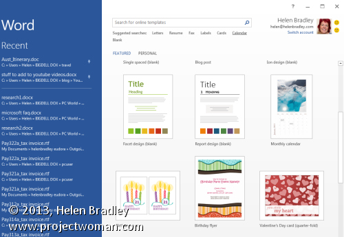
Learn how to remove the Start Screen in Word 2013
Do you hate the Start Screen in Word 2013? Many users find it cumbersome because it forces you to make a choice before continuing that many of us don’t want to have to make. Luckily it is easy to get rid of it.
If you just want to by pass it once, press Esc or Enter to open a new blank document.
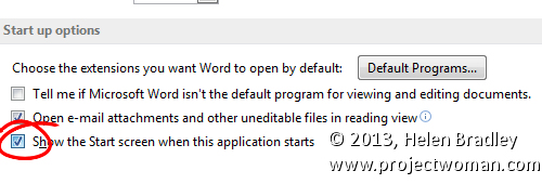
However you might want to go further and axe it permanently. To do this, launch Word and choose File > Options. In the screen there, the last option is to Show the start screen – disable the checkbox and click Ok. The start screen will be gone and, if you miss it, you can always reinstate it!

Helen Bradley
Labels: axe, disable, Hide, office 2013, remove, start menu, Word 2013, word2013
Categories:office
posted by Helen Bradley @ 12:11 pmNo Comments links to this post
Thursday, February 21st, 2013
Google Docs has the ability to use data validation to automate and manage data entry into cells in a spreadsheet. One way to do this is to limit the data that can be entered into a cell to a selection from a list that you create.
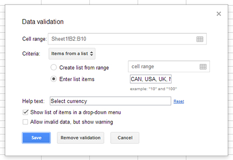
To see this at work, open an existing spreadsheet or create a new one. Select the cells into which the data will go and choose Data > Validation. From the Criteria dropdown list, select Items From a List and then click Enter List Items. Type each item for your list into the box separating entries from each other with a comma. Make sure the “Show list of items in a drop-down menu” is checked and if you don’t want a user to select anything that’s not in the list, then disable the “Allow invalid data, but show warning” checkbox. Click Save to save the validation options.

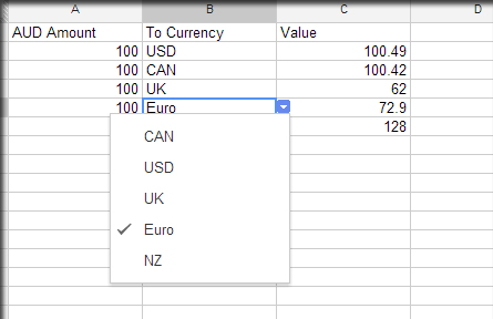
Now, when you enter data into any of the cells in the range you have configured this data validation rule for, you will see a dropdown indicator appear to the right of the cell. Click this and you can select an item from the list that is displayed below the cell. This data is entered into the cell in the same way as any data would be entered so you can, for example, use it in calculations by referring to the cell contents. In the example worksheet shown, a formula is used the cells in column C to calculate the converted value by checking what currency has been chosen and then multiplying the value in column A by the appropriate conversion rate.

It’s also possible to use other validation options using the Data Validation dialog. You can limit a cell entry to a number which meets certain criteria or to a text entry that contains or does not contain certain text or which is a valid email address or URL. You can also require that a date is entered within a certain range of dates or before or after another date.
You can force a user to comply with the data validation rules that you have created or allow them to enter an “invalid” value but warn them that they are about to enter data that doesn’t comply with the rule.
These data validation tools available in Google Docs are similar to those that you’ll find in other spreadsheet applications such as Excel.
Helen Bradley
Labels: data validation, google docs, items from a list, list, spreadsheet
Categories:hunter, office
posted by Hunter Delattre @ 9:00 amNo Comments links to this post
Wednesday, February 6th, 2013

If you’re having trouble positioning images in a document, Google provides an easy solution.
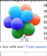
By default, all inserted images are placed inline with the text, which means it is treated just like another character and will move with the text around it. To change this, simply click on your image and select Fixed position. This places the image “above” the text so that the text moves to accommodate it; the image remains in any location you move it to while text wraps around it. This also permits images to overlap.
Helen Bradley
Labels: fit, fix, google docs, images, place
Categories:hunter, office
posted by Hunter Delattre @ 9:00 amNo Comments links to this post
Saturday, February 2nd, 2013

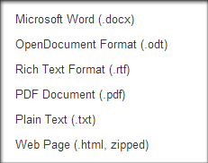
Google Docs provides a neat way of turning any document into a simple HTML web page, perfect for any novice interested in building a basic website. To do so, simply open the desired document and select File > Download as > Webpage (.html, zipped). The file will be compressed in a .zip file so you’ll have to extract it, but it will be instantly ready for use. This functionality can also be used with spreadsheets.
Helen Bradley
Labels: .html, create, download, easy, google docs, website
Categories:hunter, office
posted by Hunter Delattre @ 9:00 am1 Comment links to this post


