Monday, July 22nd, 2013

Create your first macro in Excel 2013

Learn how to type a macro in Excel 2007/2010 & 2013. Covers displaying the Developer tab and how to create your Personal Macro Workbook so you can create and save macros. Then how to create a new macro, save and run it.

Transcript:

Hello, I’m Helen Bradley. Welcome to this video tutorial. In this tutorial I’m going to show you how you can create a macro in the Visual Basic Editor in Microsoft Excel. First of all you need to make sure that this Developer tab is visible and it’s not by default. So this is Excel 2007. To make it visible you’ll click the Office button here, choose Excel Options and this is the option you want to enable Show Developer Tab in the Ribbon. With that selected the Developer tab then appears in the Ribbon. Now that’s only for Excel 2007. I’m actually going to close Excel 2007 because I’m going to work in 2010, but I just wanted to show you how you could get the Developer tab in 2007.

Now in 2010 and 2013 it’s a bit different. To get the Developer tab there you’ll choose File and then Options. And what you’re going to do is go to Customize Ribbon because only in 2010 and 2013 can you actually customize the Ribbon. And there’s an option here for Developer. So this the Developer tab and again by default it’s disabled so you want to just select it so that it is enabled and click Ok. Now this entire video was prompted by a user who asked me for a macro that would delete every row in a worksheet if there was nothing in column A.

So I have a worksheet here and I have some rows in which there is nothing at all and what we want to do is to delete them. So the first thing we need to do is to make sure that the Developer tab is visible on the Ribbon and then we’re going to actually create this macro. In fact I’m just going to copy and paste it because I just want to show you the basics of creating a macro. This might be one that you’ve been sent or it might be one you find on the web or whatever.

Now before you can actually create a macro inside the place where it’s supposed to be you have to actually have this one file created. And chances are if you’ve never created a macro before you don’t have the very file that you need. The simplest way to resolve that situation is to first before you do anything else go and click Record Macro. And you’re going to store this macro in what is called the personal macro workbook.

If you don’t have it Microsoft Excel creates it for you so that’s why we’re going to the trouble of recording just anything so that we can get this personal macro workbook created. And once it’s created then in future we’ll be able to store macros in it and these macros will always be available to every single worksheet.

Whenever Excel is opened it opens this file and everything is fine and dandy so I’m just going to click Ok. And I’m just going to type a couple of letters in there, press Enter. That’s a macro. That’s all it does and click Stop Recording. I don’t actually want the macro and I don’t actually want the contents of that cell. All I want is this special file that is called personal.xls. So I’m going to click Macros now and you can see here is the macro that we just created in this workbook personal.xls.

It’s personal.xlsb whatever it is for your particular version of Excel. And this is a file that Excel takes care of opening every time you come and open Excel so these macros are always going to be available. Now I want to add a new macro. And the macro I want to add is called remove rows. That’s just what I called it. So I’m going to type the word removerows. Now macro names have to be one whole word. You can’t use spaces but you can use underscores. I’m just going to type removerows.

And now because I don’t have that macro Excel is offering me the option of creating it. But I want to create this in my personal.xlsb workbook so I want to make sure that I select that first. Macro name personal.xlsb workbook, click Create. And what that does is it automatically opens the Visual Basic Editor for me so I don’t have to do all the work. And it also places me right in the middle of this code area which is exactly where I put my macro code. So I have it in a file so I’m just going to copy and paste it. In fact I’m going to do a little bit of the wrong thing so I can show you the result.

I’ve gone and got my file and I’ve copied the macro code to the clipboard and I’m going to paste it in. And you can see that what I did was I bought in the sub and end sub statements. And you can’t have two sets of sub and end sub statements. So the first thing I’m going to do is get rid of the extra statements. And it appears here that my lines have been cut in pieces so I’m just going to make sure that these comments are back in single lines.

So here is my removerows macro. And this has also got cut in two so let’s just neaten things up a little bit. And this is a macro that removes rows in a worksheet where the cell in column is blank. It doesn’t require you to make a selection before running it. However as Undo doesn’t work after running this macro it’s a good idea to back up your worksheet first. Well, that’s good. And I’m just going to while I’m here clean up this macro that I recorded earlier that I didn’t really want to keep but I just created so that I would get this personal.xlsb workbook.

Now that I’ve finished inside the Visual Basic Editor, I’ve created my macro I’m just going to choose File, Close and return to Microsoft Excel. Now the macro is stored not in this particular file but in this special workbook. I want to test it so the first thing I’ll do is to save my file just in case everything goes haywire. The other thing I’m going to do is just for my own purposes is format these particular rows the ones that I want to get rid of with a color. What I want to do is when I get rid of these rows the very first time I run it I just want to make sure that the macro is behaving correctly.

So if it were to do something funny I’ve marked up in orange exactly what I don’t want to see at the end of this macro. So if it were to do something like this, so let’s just go and do Delete Cells, I don’t want it to delete cells. I want it to delete a whole row so if it were to end up with something like this happening I know that my macro isn’t working. So I’m just setting myself up to check to make sure that everything is working correctly when I do run my macro. And if it works perfectly on this worksheet then I’m just going to assume that it’s going to work perfectly every other time in future.

So here we have our worksheet. Now it’s time to run the macro. Now you don’t have to use the Developer tab to do it although you can. But you can use the View tab. We’re going to Macros and here are our macros and the macros are in personal.xlsb. And the one we want to run is called removerows so I’m just going to click to run it. All the orange highlighting is gone and everything that is left are just rows that have data in column A.

So that’s how you would create a macro yourself if you found it on the web or you downloaded it from somewhere or were given it in the Visual Basic Editor in Excel. Once the personal.xlsb workbook has been created the first time you don’t have to go through that record macro step. That’s only to create that file the very first time. From now on Excel is going to take care of that file. If you’re prompted to save it when you exit Excel, say yes because you do want to save all the data that you’ve created in it. I’m Helen Bradley. Thank you for joining me for this video tutorial. Look out for more of my tutorials on this YouTube channel and visit projectwoman.com for tips, tricks and tutorials on a whole range of Office programs.

Helen Bradley

Friday, July 19th, 2013

Excel Tip – Spin Buttons for Data Entry

Learn how to use a spin button (also called a spinner) form of control in Excel to aid in data entry. Using a spin button, a user can click the button to increase or decrease a value in a worksheet cell.

This video explains how to access the Developer tab, then, how to add the spin button form control and, finally, how to set up the control. It also explains how to scale the value that the control provides so it can provide percentages and very large or very small values. This feature is in Excel 97, 2000, 2002, Excel 2007, Excel 2010 and Excel 2013.

Transcript:
Hello, I’m Helen Bradley. Welcome to this video tutorial. In this tutorial we’re going to have a look at creating spin buttons in Excel to make data entry just about as much fun as data entry can be. Before we get started with spinner controls let’s have a look and see what we’re talking about.

Here is a copy of the worksheet that we’re going to be working on and this is the spin button control. It’s been set to work between 20 and 30 so it will take a value between 20 and 30 years and every time I click the down arrow it decrements this cell by one so that the overall payment per month on the mortgage is increased because the term is much shorter. When we increase the term on the mortgage by clicking on the up arrow the overall payment is reduced. And it stops at 30.

So let’s see how we would add the spinner control to this particular worksheet.
Well first of all you have to have the Developer tab available. It it’s not choose File and then Options and in Excel 2013 and 2010 you’ll go to the Customize Ribbon button here and you’ll check this Developer tab here so that turns it on. In Excel 2007 you’ll go here because there will be an option here for Show the Developer Toolbar in the Ribbon.

So once you’ve got the Developer toolbar available click it and then take this Insert option and you want the form controls. Now the Active X controls look pretty much the same thing but they work very, very differently. And what we want are the simple form controls because they’re the easiest to use. I’m going to click here on the spin button control and then I’m going to click and drag to create the control on my worksheet. Now I can resize it later on but I’m going to start by drawing this size.

I’m now going to right click it and choose Format Control. And this gives me my options for formatting the control. To start off with I can set its current value. So I can start it at for example 25 and then I can set its minimum value which I had previously set to 20 so all our mortgages are going to tested between 20 and 30 years in length. And then I’m going to make the maximum value the 30. So we’re going to move between 20 and 30. And the incremental changes how big a change do I want to happen with each click of the button. Now these have to be integers so one is the smallest value. And cell link is a pointer to the cell that I want the value to be inserted in so I’m going to click in here and then click in this cell because this is going to be my link cell and click Ok.

You can see that the cell value changed to 25. That’s because that was the starting value. Now if I click on the spin button right now nothing is going to happen because it’s still active. So I’m just going to click outside it and now I can test it. You can see I can click up but when I get to 30 I can’t click it any more and then it will click down. And when I get to 20 it won’t go any lower.

So that’s a spin button control that you can use to control this sort of value. But there are some limits to spin buttons that we’re going to have to get around. One of them is that they only return integer values and the maximum value is 30,000. So right now that would cause us some problems in trying to add the mortgage amount which is in the region of 200,000 or more when the maximum value is 30,000. And here the interest rate is 5 percent. That’s .05. That’s not even an integer. It’s not even a one. So we’re going to have problems controlling that. And we’re going to have to find a way around it which of course can be done easily.

To see how we would deal with the situation where the amount borrowed is a much larger figure than we can use in the spin button control let’s have a look at this worksheet. In this worksheet we’re looking at how we could possibly scale a range of 0 to 30,000 to actually work for us. Let’s say that the minimum amount that we want this mortgage calculator to work for is 100,000 and the maximum is one million. Well let’s look and see what 100,000 is. Well 100,000 is 10 times 10,000 and a million is 100 times 10,000. So we could have our spinner work between 10 and 100 if we could scale it up by 10,000 each time. I’m going to replace the formula with a value and it’s going to multiply the contents of cell D2 by 10,000. Now there’s nothing in cell D2 right now but we know that we can put a value in there using a spin button.

So again Developer, I’m going to Insert and I’m going to select the Spin Button Form Control. I’m going to drag to create it on the worksheet, right click it and choose Format Control. This time I want my minimum value to be 10 because I’m going to use a 10 to 100 scale here. The maximum value is going to be 100 and I’ll have it increment by one digit at a time which is going to be 10,000. I’m going to set my current value to, for argument sake, 20 so that we’ll get back our 200,000 in this cell. And the cell link cell is going to be the cell that has the value in it that this formula is using. When I click Ok let’s see how it’s working.

As you can see the spin button here is giving us this value here of 20 and in this cell we’re just taking the value of 20 and scaling it up. So now if I click on this button it’s going up by 10,000 every click of the button and it’s going to max out at one million. And if I were to come down then it would max out in the bottom direction at 100,000. And each time as I click on the button, well I’m sitting on the button right now, but as I click on the button the amount that we’re paying each month is being recalculated accordingly. So scaling up like this is a way of getting larger values than the 30,000 that we’re allowed in the spin button control. Of course that’s preempting the solution for this value here. All we need to do now is to scale this downwards. So let’s see how we do that.

To reduce a value using a spinner we’ll work the opposite direction. Let’s say that we want an interest value between 2 and 10 percent. That’s between .02 and .1.
.02 can be represented by 2 times .01 and 10 by 10 by .01. Now that’s only going to give us whole interest values so I don’t think it’s going to be quite big enough. Let’s go down a scale and let’s say it’s 20 multiplied by .001 and 100 multiplied by .001. That’s going to give us additional percentages in the range so instead of going 2 percent, 3 percent, 4 percent we can go 2.1, 2.2, 2.3 and so on. So let’s take this scaling back to our worksheet. Again we’re going to add a spin button here so from the Developer toolbar Insert make sure that you’re using this form control and drag a spinner into position. We’ll right click it and choose Format Control and we’re going to use cell D3 as our intermediate cell. The minimum value is going to be 20. The maximum value from our previous calculations on the other worksheet is 100. We’ll use an incremental change of one for now and the cell link will be this cell here D3 and press Ok.

Now nothing is actually happening because we haven’t put our formula in here yet. The formula multiplies this value here by .001. And here is our smallest value 2 percent. We’ll need to reformat this cell so I’m going to the Home tab of the Ribbon and I’m going to increase the decimal places here so that we can see exactly what values we’re getting and not rounded values. Here everything is now going up in .1 of a percent. And it will max out at 10 percent because that’s where we set it to max out at. It won’t be able to go any larger than that.

Now all we need to do to make this worksheet a little bit neater is just to hide the column that contains those intermediary values. And now somebody can use this calculator to calculate a loan and instead of having to put value in here manually they can just click on the spin button controls to do it automatically.

I’m Helen Bradley. Thank you for joining me for this video tutorial. Look out for more of my video tutorials on this YouTube channel and visit my website at projectwoman.com for more tips, tricks and tutorials on a range of Office programs including Excel, Word, Outlook, PowerPoint and Publisher.

Helen Bradley

Thursday, July 11th, 2013

Word 2010 and 2013 Tip – Preview and Save a web page document

See your document as a web page and keep it looking that way

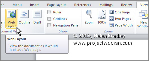
To see how any of your Word 2010 and 2013 documents will look when they are saved as web pages, select the View tab on the Ribbon, then click Web Layout.

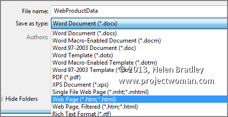
Now, to save a document as a web page, select File > Save As. In the Save As dialog, under click the Save as type: dropdown list and choose Web Page (*.htm;*.html).


Make sure to choose a location to save the document in, give it a name (it should have the .htm extension), and click Save.

Helen Bradley

Monday, July 8th, 2013

Recolor clip art in Microsoft Office 2013 and earlier

Learn to recolor clip art using theme colors so it is not only the color that you want it to be but it also matches the theme and it changes color when the theme changes.

This works with pretty much all versions of Office and all apps including Word 2013, PowerPoint 2013, Excel 2013, Publisher 2013 and older versions of Office including 2010, 2007, 2003 and earlier.

Transcript:

Hello, I’m Helen Bradley.

Welcome to this video tutorial. In this tutorial I’m going to show you how you can easily recolor clipart in Microsoft Office and how you can use theme colors so that your clipart changes when your theme changes.

Before we get started with this tutorial let’s have a look and see what it is that we are trying to achieve. This is the same piece of clipart and I just made a duplicate of that clipart image and I recolored it in the way that I’m going to show you how you can recolor your clipart. But let’s have a look and see the impact of the recoloring.

I’m going to choose the Colors tool here and watch as I arrow over all of these colors in turn. And you’ll see that the clipart image that I have recolored I have recolored this time with theme colors. And the beauty of this is that the clipart image is going to change colors in accordance with the theme that is in use.

The only thing that hasn’t been recolored is the black and the little yellow light in the candle. Everything else is a theme color and it’s going to change color using the new theme colors whenever the theme or the design of this PowerPoint presentation changes. So this is the concept that we’re going for here.

Now I have a slightly simpler image here. All I did to find these images was I chose Insert and then Online Pictures and I went looking for cake. And I particularly wanted wmf files as that’s Windows metafile and that is an illustrative file most of which can be recolored inside of PowerPoint or Word or Excel or any of the Microsoft applications.

And you don’t have to be using Microsoft Office 2013. You can choose any version of Microsoft Office. I’ve been doing this for years in Microsoft Office. It’s just that the way that you add images is a little bit different in this new version. Now before I start let’s just take a copy of this image and let’s paste it so that we’re working on a duplicate.

We can see then how far we’ve come later on. I’m just going to get rid of these images. Now with the image that I’m working on selected I’m going to choose Picture Tools, Format tab and I’m going to choose Group and then Ungroup.

Now you’ll see that the group option sometimes is not available from this dropdown menu but it will always be available from the Picture Tools, Format tab if the image is able to be ungrouped. You’ll get a message showing that this is an imported picture and not a group and asking you if you want to convert it to a Microsoft Office drawing object.

The answer to that is yes. And then you’ll go and repeat the process. You’ll right click and choose Group, Ungroup or from the Drawing Tools, Format tab you’ll choose the Group button here and choose Ungroup.

That ungroups the object so it’s now a whole lot of smaller objects. I’m just going to click outside it and then we’re going to start selecting individual pieces of this object. And I suggest that you start with a nice color scheme. So I’m just going to go to the color schemes and let’s choose something relatively colorful.

I found slip stream was a good option to use but any of these such as red violet that is fairly colorful is a good choice. Drawing Tools, Format tab and now from the shape filled dropdown list we’re going to make sure that we recolor all of the shapes using the fill colors that are theme colors.

So, again, I’m going to select here, this is on this sort of turquoise bit, and I’m going to color it a darker version of that same blue. I’m going to click on the candle light and see if I’ve got something I can use for candle light. I think I’m going to choose one of these colors because I would really like my candle light this time to be a theme color.

To select multiple colors or multiple shapes at a time I’m just selecting the first and then Ctrl clicking on the last. And again, I want these to be colored the same color as the candle light. Now I’m going to click here. There’s a shape here.

If you ever want to see what the shape is that you’re working on just press the Delete key and it will disappear and then you can undo it to be able to work on it. Or of course you can just fill it and see what it is that you are actually filling.

So I’m going to select that color. And now we’re going for this shape over here and I want a slightly darker or lighter version here. I think I’m going for a darker version. And here we have the shadows. Again, I’ll want a darker color for the shadow. I think I’ll go back for these blues. I’m going to stick to the turquoises and this sort of purple color.

So I’m going to now select these smaller items here and when I’ve got them selected I’m going to fill them as well. And when I’m pretty happy with my shape that has been recolored I’m going to select over the entire shape because now what I want to do is to stick it all back together again because I don’t want lots of little pieces.

Drawing Tools, Format tab, Group and this time I want to Regroup. And I’ll just test this by moving the object and it should all move as one. And now let’s look and see that this object is going to recolor unlike the original object if we change the color of this particular design that we’re using in PowerPoint.

So I’m going to choose the colors dropdown list here and as I choose a different color scheme you can see that my clipart shape is changing color. And as I said this works exactly the same way in any of the Office applications and in pretty near any version of these. You can do this in Word 2003.

You can do it in PowerPoint, Excel, Publisher, any of the applications and you can create clipart so that it not only matches the current theme but also looks the colors that you want it to look but which will change colors as the theme colors change.

I’m Helen Bradley.

Thank you for joining me for this video tutorial. Look out for more of my PowerPoint and Microsoft Office tutorials on this YouTube channel.

And visit my website at projectwoman.com for more tips, tricks and tutorials on a range of Microsoft Office applications as well as Photoshop, Lightroom, Illustrator and a whole lot more.


Helen Bradley

Saturday, July 6th, 2013

Explore the new Transitions in PowerPoint 2013

See the new transitions in PowerPoint 2013 including airplane and origami. There are some great new transitions and this video shows you what they are, what they look like and some of the settings for them.

Transcript:

Hello, I’m Helen Bradley.

Welcome to this video tutorial. In this tutorial I’m going to show you the new transitions in PowerPoint 2013. In this video I’m going to show you the transitions that are new in PowerPoint 2013 and we’re just going to run through them seeing them on this particular presentation. Now all of these have been in PowerPoint for some considerable time. The first of the new ones is fall over and it looks as if the slide is falling over to reveal the next slide. This is drape. Again, it’s a new transition. And curtains. This is wind.

Now with any of these transitions you can speed them up. You can see that the curtains transition takes quite a while to run but if I set it to 3 seconds then it’s going to occur a lot more quickly. Here are some more of the newer transitions, prestige. Then there’s fracture and crush and then peel off. Now like some of the other transitions this has different effect options so you can peel off from the left or the right. Then there’s page curl. And, again page curl has some different options. And airplane. The effect options for this allow you to change the direction in which the airplane flies out. And origami.

This also has effect options for the direction in which the bird flies. And finally there’s one additional transition and it’s called comb. So these are the new transitions in PowerPoint 2013.

I’m Helen Bradley.

Thank you for joining me for this video tutorial. Look out for more tutorials on this YouTube channel.

And visit my website at projectwoman.com for more tips, tricks and tutorials on various Office applications as well as for Photoshop, Lightroom, Illustrator and a whole lot more.

Helen Bradley

Wednesday, July 3rd, 2013

Word 2010 and 2013 Tip – Wrap Text Around a Table

Use a text box in Word to control text wrap around a table

In a previous tip I showed you how to place a table inside a text box so you could put two tables side by side. You can use the same process to make the text on your page wrap around a table.

Click here to learn how to place a table inside a text box

To control the way text wraps around a table, first create a text box and place a table inside it.

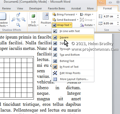
Then click to select the text box and, from the Ribbon, select the Format tab > Text Box Tools. Click the Wrap Text dropdown menu and choose the desired wrapping option from those in the list – typically you will use Square to wrap text round the text box with its inserted table.

Helen Bradley

Wednesday, June 26th, 2013

Word 2010 and 2013 Tip – Create Side by Side Tables

Place tables side by side in a document using text boxes to keep them in place

If you add a table to a text box in Microsoft Word, you can position the text box wherever you want it to be on the screen.

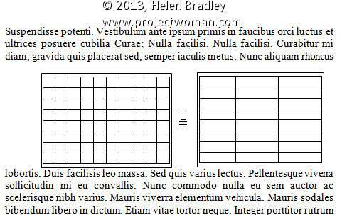
If you need two tables to be placed side by side in your document you can do so by placing each of them inside a text box and then arranging the text boxes side by side.

To do this, create a text box by selecting the Insert tab on the Ribbon, click Text Box and click Draw Text Box. Click and drag to create a text box and then click inside it and create a table by choosing Insert > Table. Repeat the process to create the second table in its text box then drag to position the text boxes side by side.

Helen Bradley

Tuesday, June 18th, 2013

Word 2010 and 2013 Tip – Colour Me Purple!

Modify a Style’s Font Color to help find missed formatting

Quickly determine which paragraphs in a document have been formatted using one style, rather than another, by changing the colour of the formatted text.

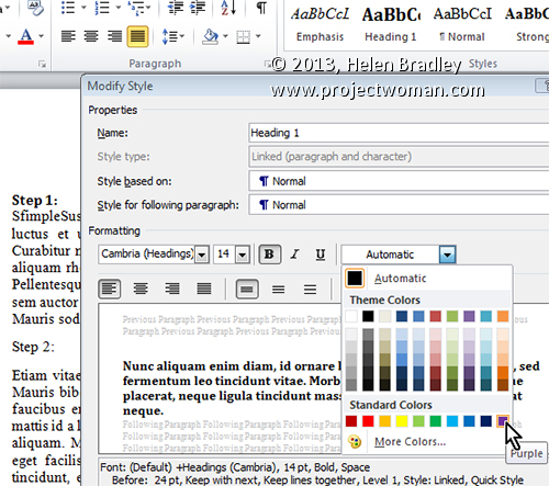
To do this, click the Home tab on the Ribbon, hover over the style’s name you want to edit in the Styles gallery. Now, right click it and select Modify. In the Modify Style dialog, change the Font Color to something that will stand out on the page (such as purple) and click OK.

Now scroll through your document to see if the style has been applied everywhere you wanted it applied. Remember, if you don’t make any changes at this point, you can quickly undo the colour change by selecting Undo.

Otherwise, when you are done formatting the document, set the colour back to the original Font Color by repeating the above steps.

Helen Bradley

Tuesday, June 11th, 2013

Word 2010 and 2013 Tip – Save documents for use with older Word versions

Learn to use ‘Save as type’ to format your document so users of older versions of Word can access them

You can easily exchange files with users of older versions of Word. This is because Word 2007, 2010, and 2013 essentially share the same file format. So it is pretty easy to open any Word document created using version 2007, 2010 or 2013 in any other of these three versions of Word. In addition, Word 2007, 2010, and 2013 will open files from any previous version of Word.

However, when you need to share a Word 2007, 2010, or 2013 file with someone using a much earlier version such as Word 2003 or a Mac version of Word, you must save the file using their particular Word file format. This is because the file formats are not the same and the older versions of Word cannot read the newer file formats.

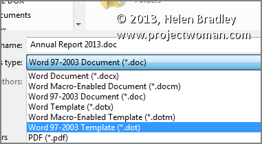
To save using the appropriate format, select the File tab on the Ribbon, and click Save As. In the Save As dialog, click the Save as type: dropdown list and select the word processing format that matches the software that your other user is using such as Word 97-2003 Document (*.doc). Then click Save to save it in that format.

Helen Bradley

Monday, June 3rd, 2013

Word 2010 and 2013 Tip – AutoNumber Table Rows

Automatically Number Any and All Rows in a Table

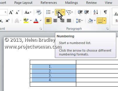
To automatically number rows in your table, select the column you wish to number (or the specific cells in the column you wish to number). Now, click the Numbering button on the Home tab on the Ribbon. After the rows are numbered, you can move the rows anywhere and the numbering will readjust automatically.

Helen Bradley