Friday, July 19th, 2013

Excel Tip – Spin Buttons for Data Entry

Learn how to use a spin button (also called a spinner) form of control in Excel to aid in data entry. Using a spin button, a user can click the button to increase or decrease a value in a worksheet cell.

This video explains how to access the Developer tab, then, how to add the spin button form control and, finally, how to set up the control. It also explains how to scale the value that the control provides so it can provide percentages and very large or very small values. This feature is in Excel 97, 2000, 2002, Excel 2007, Excel 2010 and Excel 2013.

Transcript:
Hello, I’m Helen Bradley. Welcome to this video tutorial. In this tutorial we’re going to have a look at creating spin buttons in Excel to make data entry just about as much fun as data entry can be. Before we get started with spinner controls let’s have a look and see what we’re talking about.

Here is a copy of the worksheet that we’re going to be working on and this is the spin button control. It’s been set to work between 20 and 30 so it will take a value between 20 and 30 years and every time I click the down arrow it decrements this cell by one so that the overall payment per month on the mortgage is increased because the term is much shorter. When we increase the term on the mortgage by clicking on the up arrow the overall payment is reduced. And it stops at 30.

So let’s see how we would add the spinner control to this particular worksheet.
Well first of all you have to have the Developer tab available. It it’s not choose File and then Options and in Excel 2013 and 2010 you’ll go to the Customize Ribbon button here and you’ll check this Developer tab here so that turns it on. In Excel 2007 you’ll go here because there will be an option here for Show the Developer Toolbar in the Ribbon.

So once you’ve got the Developer toolbar available click it and then take this Insert option and you want the form controls. Now the Active X controls look pretty much the same thing but they work very, very differently. And what we want are the simple form controls because they’re the easiest to use. I’m going to click here on the spin button control and then I’m going to click and drag to create the control on my worksheet. Now I can resize it later on but I’m going to start by drawing this size.

I’m now going to right click it and choose Format Control. And this gives me my options for formatting the control. To start off with I can set its current value. So I can start it at for example 25 and then I can set its minimum value which I had previously set to 20 so all our mortgages are going to tested between 20 and 30 years in length. And then I’m going to make the maximum value the 30. So we’re going to move between 20 and 30. And the incremental changes how big a change do I want to happen with each click of the button. Now these have to be integers so one is the smallest value. And cell link is a pointer to the cell that I want the value to be inserted in so I’m going to click in here and then click in this cell because this is going to be my link cell and click Ok.

You can see that the cell value changed to 25. That’s because that was the starting value. Now if I click on the spin button right now nothing is going to happen because it’s still active. So I’m just going to click outside it and now I can test it. You can see I can click up but when I get to 30 I can’t click it any more and then it will click down. And when I get to 20 it won’t go any lower.

So that’s a spin button control that you can use to control this sort of value. But there are some limits to spin buttons that we’re going to have to get around. One of them is that they only return integer values and the maximum value is 30,000. So right now that would cause us some problems in trying to add the mortgage amount which is in the region of 200,000 or more when the maximum value is 30,000. And here the interest rate is 5 percent. That’s .05. That’s not even an integer. It’s not even a one. So we’re going to have problems controlling that. And we’re going to have to find a way around it which of course can be done easily.

To see how we would deal with the situation where the amount borrowed is a much larger figure than we can use in the spin button control let’s have a look at this worksheet. In this worksheet we’re looking at how we could possibly scale a range of 0 to 30,000 to actually work for us. Let’s say that the minimum amount that we want this mortgage calculator to work for is 100,000 and the maximum is one million. Well let’s look and see what 100,000 is. Well 100,000 is 10 times 10,000 and a million is 100 times 10,000. So we could have our spinner work between 10 and 100 if we could scale it up by 10,000 each time. I’m going to replace the formula with a value and it’s going to multiply the contents of cell D2 by 10,000. Now there’s nothing in cell D2 right now but we know that we can put a value in there using a spin button.

So again Developer, I’m going to Insert and I’m going to select the Spin Button Form Control. I’m going to drag to create it on the worksheet, right click it and choose Format Control. This time I want my minimum value to be 10 because I’m going to use a 10 to 100 scale here. The maximum value is going to be 100 and I’ll have it increment by one digit at a time which is going to be 10,000. I’m going to set my current value to, for argument sake, 20 so that we’ll get back our 200,000 in this cell. And the cell link cell is going to be the cell that has the value in it that this formula is using. When I click Ok let’s see how it’s working.

As you can see the spin button here is giving us this value here of 20 and in this cell we’re just taking the value of 20 and scaling it up. So now if I click on this button it’s going up by 10,000 every click of the button and it’s going to max out at one million. And if I were to come down then it would max out in the bottom direction at 100,000. And each time as I click on the button, well I’m sitting on the button right now, but as I click on the button the amount that we’re paying each month is being recalculated accordingly. So scaling up like this is a way of getting larger values than the 30,000 that we’re allowed in the spin button control. Of course that’s preempting the solution for this value here. All we need to do now is to scale this downwards. So let’s see how we do that.

To reduce a value using a spinner we’ll work the opposite direction. Let’s say that we want an interest value between 2 and 10 percent. That’s between .02 and .1.
.02 can be represented by 2 times .01 and 10 by 10 by .01. Now that’s only going to give us whole interest values so I don’t think it’s going to be quite big enough. Let’s go down a scale and let’s say it’s 20 multiplied by .001 and 100 multiplied by .001. That’s going to give us additional percentages in the range so instead of going 2 percent, 3 percent, 4 percent we can go 2.1, 2.2, 2.3 and so on. So let’s take this scaling back to our worksheet. Again we’re going to add a spin button here so from the Developer toolbar Insert make sure that you’re using this form control and drag a spinner into position. We’ll right click it and choose Format Control and we’re going to use cell D3 as our intermediate cell. The minimum value is going to be 20. The maximum value from our previous calculations on the other worksheet is 100. We’ll use an incremental change of one for now and the cell link will be this cell here D3 and press Ok.

Now nothing is actually happening because we haven’t put our formula in here yet. The formula multiplies this value here by .001. And here is our smallest value 2 percent. We’ll need to reformat this cell so I’m going to the Home tab of the Ribbon and I’m going to increase the decimal places here so that we can see exactly what values we’re getting and not rounded values. Here everything is now going up in .1 of a percent. And it will max out at 10 percent because that’s where we set it to max out at. It won’t be able to go any larger than that.

Now all we need to do to make this worksheet a little bit neater is just to hide the column that contains those intermediary values. And now somebody can use this calculator to calculate a loan and instead of having to put value in here manually they can just click on the spin button controls to do it automatically.

I’m Helen Bradley. Thank you for joining me for this video tutorial. Look out for more of my video tutorials on this YouTube channel and visit my website at projectwoman.com for more tips, tricks and tutorials on a range of Office programs including Excel, Word, Outlook, PowerPoint and Publisher.

Helen Bradley

Sunday, March 31st, 2013

Excel – Create a button to move to another sheet in the Workbook

Create a button in Excel to move the user to another worksheet

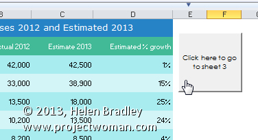
It is easy in Excel to create a button on a worksheet that you can click to go to another sheet in the workbook. It is also a fun way to get started with macros in Excel if you have never made one before.

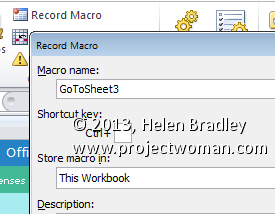
To do this, first decide which sheet will contain the button and which sheet you will select when you click, the button. We’ll add a button to sheet1 to take us to sheet3. So, click in Sheet 1 and, from the Developer tab on the Ribbon, choose Record Macro. If the Developer tab is not visible click here to find out how to display it.

Type the Name GoToSheet3 (a macro name must be all one word) and from the Store Macro in List choose to store the macro in This Workbook and click Ok.

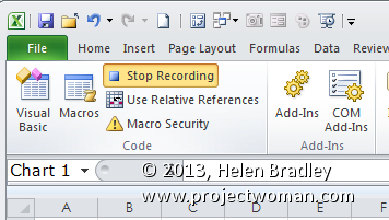
Click the tab for Sheet 3 and then click Stop Recording on the Developer tab. The macro will be recorded and stored automatically for you.

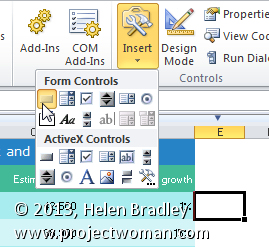
To add a button to Sheet 1 that will run the macro, first return to Sheet 1 and from the Developer tab on the Ribbon select the Insert option and click the Button (Form Control) option at the top of the drop down list. You must choose the Form Controls and not the Active X Controls.

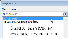
Drag a button onto the worksheet and when the Assign Macro dialog appears, click the GoToSheet3 macro and click Ok.

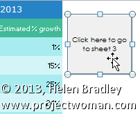
Select the text on the button and type Click to go to Sheet 3.

Click outside the button to unselect it and then click on the button to see it at work. When you click it you will be taken automatically to sheet 3.

If you need to make changes to the text on the button right-click on it to get access to the text. You can’t click it to select it because clicking it runs the macro attached to it.


Helen Bradley

Monday, March 25th, 2013

Excel – What to do when PivotTables won’t total


When Excel won’t total a PivotTable there is a reason why – and a workaround

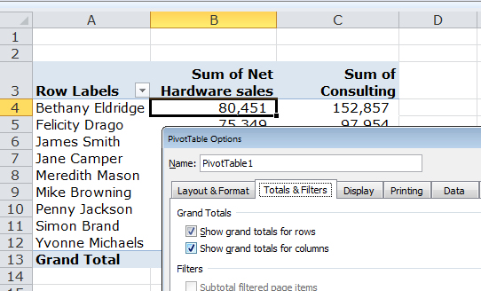
When you are working with a PivotTable in Excel and if the data you are looking at comes from two different columns in the original worksheet you won’t be able to create automatic totals for it in the PivotTable.

So, as much as you ask Excel for totals, you’ll be disappointed.

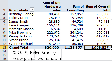
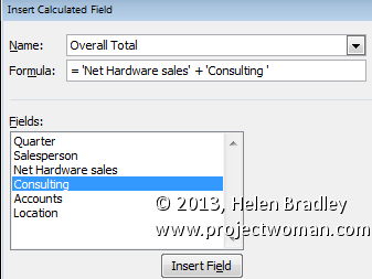
However, you can create manual totals. To do this, click in the table and from the Options tab choose Fields, Items & Sets > Calculated Field. In the dialog, click in the Name box and type the name Overall Total. Click in the Formula box and write a formula that totals the fields you want to total. In our example it will be Net Hardware Sales plus Consulting.

To write the formula click next to the = symbol in the Formula box. Click Net Hardware Sales in the Fields box and click Insert Field. Add a + symbol to the formula, then click Consulting in the Fields box and click Insert Field.

The resulting formula will read: = ‘Net Hardware sales’ + ‘Consulting ‘

When you are done, click Ok and the calculated field will be added to the table and it will be visible alongside the other fields in the PivotTable.

Helen Bradley

Tuesday, March 19th, 2013

Excel – Sum a cell in all sheets but this one

Try this quick Excel formula to sum a cell in all the sheets except the current one

In Excel sometimes you’ll want to sum a cell value in all the sheets except the one that you’re currently working on. You might do this if you have a series of quarterly results that you want to add together to create a yearly total in the total sheet.

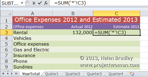
You can do this by typing the sheet name and cell for each cell to add but that would be very cumbersome. It will be a nuisance too if you try to select each cell in turn. Luckily Excel has a special feature that will help you do this. So, to sum all the values in, for example, cell C3 of every sheet in the current workbook except for the sheet you are currently working on, use this formula:

=SUM(‘*’!C3)

The ‘*’! part of the formula tells Excel that it should total all the sheets in the workbook except the current worksheet. When you press Enter Excel expands the formula so it will refer to the first and last sheets in the workbook. So, if you are summing that cell in a workbook that has sheets called YearTotal, Quarter1, Quarter2, Quarter3, and Quarter4 the formula will be expanded automatically so it reads:

=SUM(Quarter1:Quarter4!C3)

Be aware that if you add additional sheets to the workbook which appear inside the range of the sheets that are refered to in the formula then those additional worksheet cells will be included in the total.

If you don’t want this to be the case then make sure that any new sheets that you add appear outside the range of sheets that are included in the formula.

Helen Bradley

Friday, March 15th, 2013

Motion charts in Google Docs

Gadgets allow you to do things with Google Docs that would be time consuming if not beyond most people’s skills to create in a program like Excel. In this article I’ll demonstrate how to create a motion chart in Google Docs spreadsheet.

Prepare the data
In the first column of a new worksheet type the name of the item you’re charting such as office locations – we’ll use City and Bayside. In the next column, type the period that the data is for – this needs to be a time field such as year, week or quarter. The data needs to conform to ISO8601 so use 2011 for a year, 2011W08 to enter week eight of 2011 or 2011Q2 for second quarter 2011.

In the next column, type the data to plot such as Profit. The next columns are optional but we’ll add one which records units sold. To have some data to work with, add at least five years of data for the two offices.

Add the Gadget
Select over the entire range (including headings), and choose Insert > Gadget > Charts and scroll to find the Motion Chart and click Add to Spreadsheet. In the dialog which appears, the range should already cover the selected range, leave the Default State empty for now and type a title for your chart such as 5 Year Office Comparison and click Apply & Close.

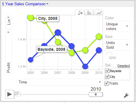
The chart appears on the screen but requires some customisation to  work. From the fly out menu of Y axis options on the left select Profit and then from the X axis dropdown list select Time so you plot Profit against Time.

From the Color dropdown list, select Unique Colors and from the Size dropdown list, select Units Sold.

Click the Play button and the chart will play showing the change in your data over time. The Y axis movement shows movement in Profit and the size of the bubble shows change in Units Sold.

The tabs change the chart from a Bubble to a Column or Line (this is not a motion chart).

If you click the office checkboxes and Trails you will see additional labels on your data and to the right of the Play button is a slider which controls playback speed.

Save the default
Wind the play button back to the beginning. Click the Settings button and click Advanced and Advanced again. Double click the state string to select it, right click and choose Copy. Click the chart title to display the chart menu, click Edit Gadget and paste the string into the Default State textbox. Save the worksheet and the chart will appear whenever the worksheet is viewed and it will be configured as you set it up to look.


Helen Bradley

Tuesday, November 20th, 2012

Trevor’s Quick Excel Tip – Display Formulas

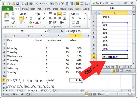
When you need view formulas instead of their results press Ctrl + ~ to display formulas in all cells in the worksheet. To return to viewing the worksheet as it was, press Ctrl + ~ again.

Helen Bradley

Tuesday, November 6th, 2012

Trevor’s Quick Excel Tip – Select Everything

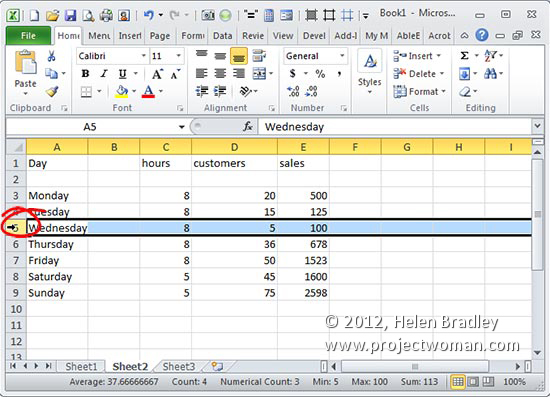
To select an entire row or column in an Excel worksheet, click the column letter or the row number. To select multiple columns or multiple rows click and drag over the column letters or row numbers to select. To select the entire worksheet, click the empty box at the intersection of the Rows and Columns in the top left of the worksheet.

Helen Bradley

Thursday, October 18th, 2012

Holiday Gift Budget Worksheet

Don’t blow the budget this holiday season!

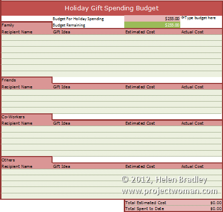
Our holiday gift buying budget worksheet will help you avoid a Yule tide spending blow out.

In the interests of helping you better control your spending this Holiday Season we have a free spreadsheet download in the form of a Holiday Gift Spending Budget.

Grab this version for Excel 2007/2010/2013 – gotta love the formatting available in those versions.

If you’re stuck in the land of Excel 2003 and earlier (or want to use it in Zoho, Google Docs, OpenOffice.org or anything else that can read Excel files), then grab this plainer but still fully functional version.

The worksheets are protected against wiping out key formulas and entering data in the wrong cells but there’s no password there so you can easily unprotect if you desire.

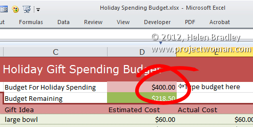
To use this worksheet, download the one for your Excel version, open it in Excel (or another compatible program), and then, in cell D2 type the amount you can afford  to spend.

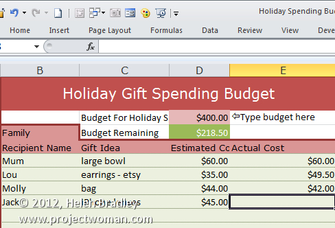
Then add entries for family, friends, co-workers and others – determine what you will get them and  how much you are budgeting to spend. At this stage you can see if you are on track or already over budget.

As you buy presents, fill in the actual amount spent and in cell D3 you will see what you still have to spend of your budget amount or if have spent all you have allowed for.


Helen Bradley

Tuesday, October 9th, 2012

Trevor’s Quick Excel Tip – Date and Time

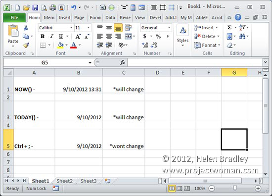
To enter the current date and time into a worksheet cell type =NOW() to display both the date and time based on the regional options that are set for your copy of Windows.  If you want the date and not the time, type =TODAY(). These formulas update themselves every time Excel is opened, the worksheet is recalculated or if it is printed.  If you need to enter the current date or time so it is fixed and so it won’t change, press press Ctrl + ; for the date or Ctrl + Shift + ; for the time.

Helen Bradley

Tuesday, September 18th, 2012

Trevor’s Quick Excel Tip – Navigate cells

Move around the cells in your workbook without touching your mouse using the Up and Down and Left and Right Arrow keys. To jump to the edge of the current block of data press Ctrl + the appropriate arrow key – so to move to the last row press Ctrl + Down Arrow.

Helen Bradley

Page 2 of 41234