

When you’re working with a large worksheet where the data appears in rows across the sheet, you may find it difficult to keep track where you are as your eye moves across a row. You can solve this problem by formatting each alternate row in the worksheet a different colour.
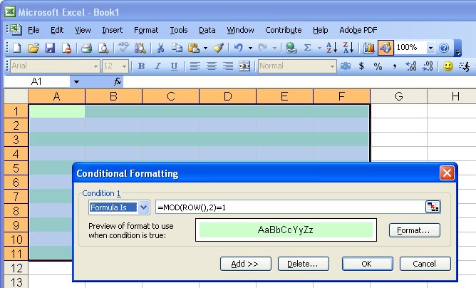
Select the entire worksheet, or just the area containing the data, and choose Format, Conditional Formatting. From the first dialog choose Formula Is and, in the text area to its right, type =mod(row(),2)=1. Click the Format button and set the format to use for each alternate row in your worksheet (a light pastel colour is a good choice). Click Ok twice and each alternate row in your worksheet will be formatted accordingly.
You can apply the same concept to formatting alternate columns if this is the way you view the worksheet. In this case use -=mod(column(),2)=1.
This formula uses the MOD function which calculates the remainder when the current row number is divided by 2 and then tests to see if it is equal to 1. If it is, then the row is formatted, if not, it isn’t. For the first row, the remainder when the row number (1) is divided by 2 is 1 and that is equal to 1 so the answer is true and the format is applied to the first row. The same result happens for each odd numbered row (any odd number divided by 2 gives a remainder of 1). For even numbered rows, there is no remainder so 0=1 is a false statement and the format is not applied.
Post a Comment
Please feel free to add your comment here. Thank you!