Monday, September 17th, 2007

Error Checking in Excel

Chasing problems in Excel worksheets is a major pain. It helps to create them accurately in the first place but when you’re trying after the fact, to find problems, Excel has some tools that can help. One of these is the often overlooked Go To option.

Go To can find formulas that vary from those in the cells that surround them. This can help you find formula errors which would otherwise be difficult to locate.

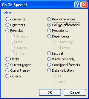
So, for example, if you have a column of cells which should all contain the same formula you can check to make sure they are written the same way by selecting the cells and choose Edit, Go To, Special, Column Differences (in Excel 2007, from the Home tab select Find & Select, Go To Special and then click Column Differences). Any cells which contain a formula that relates to a different series of cells to those in the active cell will be selected so you can check them. The Row Differences option does the same thing for rows of cells.

Helen Bradley

Friday, September 14th, 2007

How-To with Helen Bradley

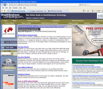
I write for lots of wonderful publications across the globe and one of them is Internet.com’s Small Business Computing web site.

The great news is that I now have my own section and here it is: SmallBusinessComputing.com. Check a few sections down and you’ll see a link to all my small business columns. There are heaps of columns on all things Office including Office 2007 and lots of stuff for earlier versions too. It’s a great way to get down and dirty with some of the new features in Excel, PowerPoint and Word including Themes, SmartArt, Charts and lots of other handy tools.

Helen Bradley

Friday, August 24th, 2007

Excel 2007 – Now where to?

When I enter data across a row in Excel it is extremely annoying when the cell pointer moves down instead of across when I press the Enter key. Luckily I know how to make it work for me and in a couple or four steps, it’s doing what I want.

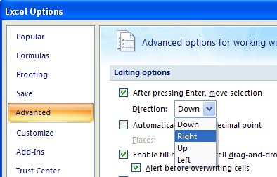
Click the Office Button, click Excel Options, Advanced and the first entry in the list is what you want. From the dropdown list select the movement option to use for the mouse and click Ok to end. Alternately disable the checkbox and the cell pointer won’t move at all.

It’s simple enough a process that you can change it whenever it suits you to do so.

Helen Bradley

Tuesday, August 21st, 2007

Splitting data in Excel

Let’s set the scene. You have a column in an Excel worksheet which contains a list of names, first name and last name all together. You want to split these into two columns, one for First name and one for last. How do you do this? Well one way is to use the Excel Text to Columns option.

Start by inserting a couple of columns to the right of the column which contains the names. Select the column containing the names and, in Excel 2007, click the Data tab on the Ribbon and choose Text to Columns. Step through the Wizard. In the first step choose Delimited and in Step 2 choose Space. Click Finish and answer Yes to the prompt to overwrite data. You will now have the data in two columns. You’ll be able to remove the extra column you have there – it’s best to add too many blank columns and later remove those you don’t need because if you don’t, you’ll run the risk of losing the columns to the right of where you are working.

This is a simple and very fast solution for a name splitting problem.

Helen Bradley

Friday, August 17th, 2007

Status bar functionality – Excel 2007

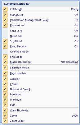
Right click the Status Bar in Excel 2007 and an entire grab bag of options open up for your choosing. You probably already knew that you could configure Excel in earlier versions to show you a single calculation on a selected range of cells – so you could select cells and then read the Sum of the values on the Status Bar (you did know that didn’t you?) but the functionality is even better in Excel 2007.

Here you can choose to view an entire range of calculations so, instead of being forced to choose between Sum and Average you can have both display and throw in Min, Max and Count for good measure too!

You can also add a Macro Record button to use to fire off the Macro recording tool without having to delve into the ribbon to do so.

It all adds to your very slim customization pickings in Excel 2007 – make the most of it, this and the Quick Access toolbar are about all you’ve got to play with.

Helen Bradley

Thursday, July 12th, 2007

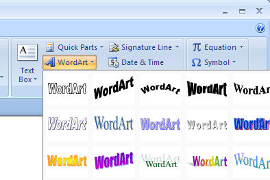
Don’t look now! WordArt in Word 2007

If you’ve tried the new WordArt tool in PowerPoint 2007 you’ve probably discovered how neat it is. No more bent words in putrid magenta colors and instead, theme aware text that looks great for headings and which will change color when you change the Theme.

Try the same thing in Word 2007 and you’re in for a ghastly surprise. WordArt missed out on getting a makeover in Word 2007 and, instead, it’s the same application it has always been – functional but requiring a lot of additional work on behalf of the user to make it look even half good.

Here’s hoping that the next implementation of Word, whenever that appears, finally does away with this and gives us WordArt that is usable and as functional as that in PowerPoint 2007 and Excel 2007.

Helen Bradley

Saturday, July 7th, 2007

Close everything NOW! Excel 2007 and PowerPoint 2007

Yum, it’s like a boss key for Excel and PowerPoint. Double click the Office button in either application and it’s like a Close All tool – everything closes quickly and automatically.

Doesn’t work in Word, wonder why not?

Helen Bradley

Wednesday, June 20th, 2007

Millions in Excel

Excel has some cool formatting tricks up its sleeve and one of these is its ability to shrink really big numbers down to size.

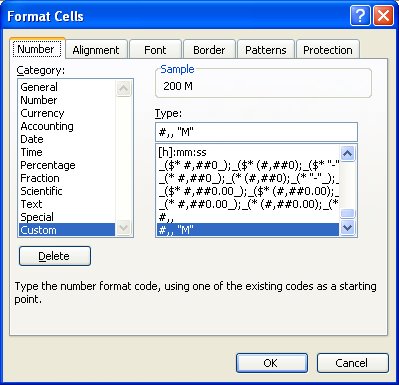
So, if you have values in the millions – like your salary – Ha!, you can size them down to size using a custom format. Select the cells, choose Format, Cells, Number tab and click the Custom group and type #,,”M” and Excel will format 200,000,000 to read 200M! The numbers aren’t altered it’s just a simpler way of displaying them.

Since the Y axis of a chart inherits its formatting from the top left cell in the chart data range this lets you format a chart’s Y axis to show the smaller values too.

Helen Bradley

Wednesday, June 13th, 2007

Changing Excel 2007 Default template location

Q: Where do you go to change the default locations for templates in Excel 2007?

Luckily I already know the answer to this question because my bet is that it’s going to take your hours to work out how to do it. You see, there’s no way in Excel to change the default location for where its templates are stored, in particular as one of my blog readers found to his chagrin, the default location for saving chart templates.

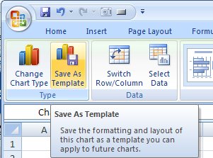
Perhaps I’ll start this story again, this time at the beginning. In a recent blog entry I showed you how to save a chart template. The process is this: create your chart in Excel 2007 and then from the Design tab which appears only when you have the chart selected, click the Save As Template button in the Type group and save your file in your default templates folder which should be c:\Documents and Settings\username\application data\Microsoft\templates. The file should have the .crtx extension.

Close your Excel worksheet, close Excel, open Excel again, create the data for a new chart, select the data and choose Insert, Other Charts, All Chart types, Templates and your chart template should appear in the list. So far so good.

Problem is that not everyone’s installation of Excel 2007 looks to this default location for either saving chart templates or finding them when you need to use them. In particular you may confront this problem if you’re on a network. So the question then becomes where are your chart templates supposed to be saved to? Answer – who knows? You see, there’s no setting in Excel to say where to put them, so you have no clue where Excel is looking for them, so you can’t put them there because where is “there”?

So, we’re now at the point where we know there’s no setting in Excel for specifying the default location for templates. If we could set this, we could save our template there and Excel could find it… simple to understand, but problematic to achieve.

The solution that I found and which works is to make the change in Word 2007 – not exactly the first place you’d look huh? If you visit this link: www.kbalertz.com/kb_924460.aspx you’ll see buried in the KnowledgeBase article quoted there, information on how the template locations in Office 2007 programs are managed.

There are some registry entries that you can change but the simpler solution is to change the location in which your templates are stored using the Word settings. When you use Word 2007 to change the location where your Word templates are stored you also change the location where all Office 2007 templates are stored. So Word’s settings control every other program which is sort of handy to know because you could spend all day looking in Excel for a place to change the Excel template location.

So here’s the short information on how to change Excel’s default template locations: —

Start Word 2007, click the Office button and choose Word Options, Advanced and locate the General group. Click File Locations, User Templates, Modify and in the modify location dialog change the setting in the folder name list or the look in list to point to the folder where your templates will be saved.

For ease of access and backup I suggest that you put it where they were supposed to be put in the first place which is Documents and Settings\username\Application Data\Microsoft\templates but theoretically you could put them anywhere.

This changes the setting in the Windows registry so that all templates are now saved to this location.

The KnowledgeBase article makes essential reading for anybody trying to manage Microsoft Office applications particularly in a network situation.

Helen Bradley

Tuesday, May 22nd, 2007

Quick moves in Excel

My friend Theda and I were talking the other day about a project she’s working on where she has to reorder a lot of items into alphabetical order and, in some cases, an order which is not alphabetical.

While she is doing the project in Microsoft Excel there are, of course, difficulties in Excel in moving items around as Excel does not, by default, open up a row when you choose to move an item from one part of the worksheet to another – instead, Excel thinks you want to overwrite the target cells – as if!

There is, however, a way to do this which opens up the space for the new row and which closes up the space that you have just made available. To do this select an entire row or range of rows in Excel by clicking on the row number or numbers. Hold your mouse over the dark outline around the rows and hold the Shift key as you drag the rows to their new position. The empty space that you have created will be closed up and a new space will be created between the other two rows for your item.

Problem solved!

Helen Bradley

Page 4 of 512345