Friday, July 20th, 2012

Here are five cool tips, tricks and keystrokes to help your day go faster in Excel:
Display cell formulas and not results
If you want to see the cell in your worksheet display formulas rather than the results of those formulas then you can do it one of two ways.
Use the keyboard shortcut Ctrl + ~ to toggle formula display on and off
You can also use Formulas > Show Formulas

Start a new line
When you need to add a line break to a cell to start a new line of text press Alt + Enter in the cell. If you just want to wrap a long piece of text in a cell right click the cell and choose Format > Alignment tab > Wrap Text.

Copy the contents of the cell above
To copy the contents of the cell above into the current cell press Control + ‘.
Moving around super fast and super smart
To move from one sheet in a workbook to the next (or in reverse), press Control + PgDn and Control + PgUp. To move to the next open workbook press Control + Tab or Control + Shift + Tab.
Super quick mouse free SUM formula
Skip taking the mouse to your Ribbon to add a SUM function and do it with a simple keystroke instead. Type Alt + = and Excel adds the SUM function automatically to the current cell. Doesn’t get much easier than that!
Helen Bradley
Labels: cool, copy formula, Excel 2007, Excel 2010, excell, format, Helen Bradley, keystrokes, line break, new line, shortcut key, show formulas, sum function, techniques, tips, tricks, Wrap text
Categories:office
posted by Helen Bradley @ 7:34 am9 Comments links to this post
Thursday, April 12th, 2012

The Quick Access Toolbar or QAT runs across the top left edge of the Word 2007 and 2010 window. It also appears in other ribbon compatible programs like Excel 2007 & 2010, PowerPoint 2007 & 2010.
The QAT is a handy place to put icons that you use all the time. It can be customized through this Quick Access Toolbar option.

Click this icon to show the QAT editing options. Click Show Below the Ribbon to place the Quick Access Toolbar below the ribbon – I think most people will find its current position acceptable but if you want to move it that’s how to place it elsewhere.
Choose More Commands to add more commands to the Ribbon. From the Choose Commands From list you can select commands to view. These include Popular Commands, Commands Not In The Ribbon, in other words commands that are available in Microsoft Word but for which you have no other easy way of accessing, All Commands or Macros. The remainder of the dialog gives you access to the individual tabs in Word so that you can get access to icons listed there.

Some options you may want to add to the Quick Access Toolbar include the Close/Close All Button, Quick Print and I like to add Switch Windows which is available from the All Commands list. Other tools that you use frequently can be added to the Quick Access Toolbar making them instantly accessible.
You should note that you can set the features for all documents or for just an individual document so that you can, for example, set a different toolbar for a specific document. When you choose this option the specific document will get all the tools on the standard quick access toolbar plus those that you’ve added to just its toolbar.

Helen Bradley
Labels: Excel 2007, Excel 2010, Helen Bradley, mini toolbar, OneNote 2010, Outlook 2010, PowerPoint 2007, PowerPoint 2010, Qat, quick access toolbar, Ribbon, Word 2007, Word 2010
Categories:Uncategorized
posted by Helen Bradley @ 8:00 am1 Comment links to this post
Tuesday, January 10th, 2012

In Excel 2003 and now in Excel 2010 , there are pattern fills which you can use to fill chart bars so your charts print just great in black and white.
Unfortunately the same feature was removed from Excel 2007 – wtf? I have no clue why but it was but it has to be a very silly thing to have done.
If you are using Excel 2007 and you need to use pattern fills with a chart you are out of luck – well not really – you just need to read the rest of this tip because I can tell you how to put the fills back into Excel 2007.
To begin, download this handy add-in: http://officeblogs.net/excel/PatternUI.zip
Update: This link is no longer live so patternui.zip is not longer available. You can find an add-in here (with instructions which achieves the same thing) courtesy of Andy Pope.
The zip file contains a single file patternUI.xlam which you need to extract and place somewhere you will find it easily and where it won’t get deleted by accident. You could make an Excel add-ins folder for it, for example.
Once you’ve done this, open Excel 2007 and choose the Office button > Excel Options > Add-ins and from the Manage dropdown list, select Excel Add-ins and click Go. This opens the old Add-ins dialog from earlier versions of Excel. Click Browse and locate the .xlam file that you just unzipped and placed somewhere safe. Select it and click Ok. Ensure that the PatternUI option appears in the Add-ins available list and that it is checked and click Ok.
Now create an Excel chart. Once you have you chart, click on the data series to fill with a pattern – if you have a single series plotted then select just one of the columns at a time. Select the Chart Tools > Format tab and notice that you now have an option called Patterns available. Click the Patterns option and select a pattern to apply to the currently selected chart series or column. Click on each series or column in turn and apply a pattern to it. When you are done, you can print your chart as usual.
Installed add-ins are managed automatically by Excel so you will find that the add-in will still be there and accessible next time you use Excel.
If you are using Excel 2010 you don’t need this add-in as the pattern fills are back where they should have been all the time.

Helen Bradley
Labels: add-in, black and white, charts, download, Excel 2007, Excel 2010, free, pattern fills
Categories:Uncategorized
posted by Helen Bradley @ 9:55 am36 Comments links to this post
Wednesday, October 12th, 2011

Often you will want to extract a month or day of the week from an Excel date. This is extraordinarily easy to do using the text function.
To get the name of the day of the week from a date in, for example, cell A1 type this into another cell:
= TEXT(A1,”dddd”)
This will give you the full day name spelled out such as Monday or Tuesday.
If you want a three character name use:
= TEXT(A1,”ddd”)
The same basic formula can be used to get the month of the year from a date. Use this to get the month name spelled out in full:
= TEXT(A1,”mmmm”)
Use this to get the month of the year spelled out in three characters:
= TEXT(A1,”mmm”)
and this for a single letter month:
= TEXT(A1,”mmmmm”)
This formula can be easily constructed and copied down a column of dates to extract just the information you want very quickly and easily.
The Excel help file has some information about the different formats you can use to extract data using the TEXT function.

Helen Bradley
Labels: day of the week from a date, Excel 2007, Excel 2010, functions, month name from a date
Categories:Uncategorized
posted by Helen Bradley @ 9:13 am10 Comments links to this post
Thursday, October 6th, 2011

Hmmm … I am fussy, I want my cake and I want to eat it too!
I want to have a clean task bar so I don’t want to see lots of files lined up there so I love Windows 7 and its clean task bar. But I find the new panel that opens when I right click an icon on the task bar to be just a little bit too free with information. I really want it to show me a list of currently open files – not everything that I have open or have recently opened. Actually I could live with the information it gives me if I didn’t have to actually use it to switch windows.
So, problem is… how can I switch between open documents in Excel or Word, for example, without having to use the Windows task bar? Solution is to use the Switch Windows button. I add it to the QAT (Quick Access Toolbar) and it totally makes sense to me.
In Excel or Word, click the Customize Quick Access Toolbar button and choose More Commands. From the list which currently shows Popular Commands choose All Commands and scroll to find the Switch Windows button and click Add.
Now it is on the QAT and it will show you all your open files and you can use it to switch between them by just clicking on the one to go to. Repeat the process for both Excel and Word and you’ll be happy – at least until something else bugs you!
Helen Bradley
Labels: Excel 2007, Excel 2010, filenames on task bar, Switch between open documents, switch between open worksheets, Windows 7, Word 2007, Word 2010, workbooks
Categories:Uncategorized
posted by Helen Bradley @ 8:58 am3 Comments links to this post
Monday, October 3rd, 2011

Consider this scenario – you have a cell which contains a link to data in another cell on another sheet. The link might be the only thing in the cell or it might be a link in a formula which contains references to data in lots of other cells too.
If you want to go to a particular referenced cell you could read off the cell details – its sheet name and its cell reference and navigate there yourself or you could get smart and have Excel do the work.
To do this, click in the cell containing the reference and choose Formulas > Trace Precedents. When you do this you will see a small sheet icon and an arrow with a black arrow head pointing at the cell. Hold your mouse cursor over the arrow until the mouse cursor turns into a hollow white arrow. Double click and the Go To dialog will open. In it will be references to all the cells in the formula. Click the reference you are interested in going to and the cell reference will be highlighted – click Ok and Excel will take you direct to that cell.
If you have both workbooks open the same process will work to take you to a cell in another workbook if it is referred to in a formula in the current workbook.
Helen Bradley
Labels: Excel 2007, Excel 2010, go to a cell, go to a cell on another sheet, go to a cell on another workbook, trace precedents
Categories:Uncategorized
posted by Helen Bradley @ 9:45 am1 Comment links to this post
Sunday, June 5th, 2011
 Some things Microsoft does make no sense at all. For this read showing the Developer Tab in Excel 2010. Ok first of all why hide the damn thing. Second of all why change how it is displayed from Excel 2007 to 2010 – yep they did – and yep it makes NO sense to do so.
The Developer tab contains some sweet goodies like form tools which let you put a button on a worksheet to run a macro – but you won’t know you can do this till you show the Developer tab.
Ok… here’s how: Click the File button and click Customize Ribbon. In the left panel is the Developer toolbar but its checkbox is deselected. Click to check it and Voila! you now have a Developer tab.
In Excel 2007, skip; the fuss – there is no Customize option and the option to display the Developer toolbar is in the first panel you see in the Excel Options dialog.

Helen Bradley
Labels: Developer toolbar, Excel 2007, Excel 2010
Categories:Uncategorized
posted by Helen Bradley @ 7:54 pm3 Comments links to this post
Friday, April 29th, 2011

In Excel 2003 and earlier you might recall that you could click a cell and choose Edit > Clear and choose to clear its Contents, Comments, Formatting or choose All to remove everything.
In Excel 2007/2010 there is a Clear Contents option on the right click menu but, in the absence of the Edit menu you’ll need to look elsewhere for the other options. On the Home tab of the Ribbon look for the Clear icon – it has an eraser on it and it has a dropdown list from which you can select the desired option.
It’s pretty obvious if you’re using Excel at full screen size but shrunk down it isn’t clear (pun intended) that it is there or what it does. I like to add the Clear All option to the Quick Access Toolbar so it’s easy to find and use. You will find it in the All Commands list and it is called Clear All if you’re looking for it.
Helen Bradley
Labels: delete cell contents, Excel 2007, Excel 2010
Categories:Uncategorized
posted by Helen Bradley @ 9:05 amNo Comments links to this post
Wednesday, June 16th, 2010
 If you are having difficulty understanding how a formula is calculating in Excel – perhaps because it appears to give you the wrong results – you can step through it to see how it is working.
To do this, select the cell containing the formula and choose Tools > Formula Auditing > Evaluate Formula – in Excel 2007 find the Evaluate Formula option on the Formulas tab.
Click Evaluate and each time you do this, a portion of the formula will be evaluated and you can see it at work.
Use the Step In and Step Out options to see the actual values in place of any appropriate cell references.
This step by step processing should show you what is happening in your formula allowing you to troubleshoot any difficulties with it.
Helen Bradley
Labels: Excel 2003, Excel 2007, Excel 2010, Excel formulas, formula auditing, troubleshoot
Categories:Uncategorized
posted by Helen Bradley @ 7:04 am4 Comments links to this post
Thursday, November 5th, 2009
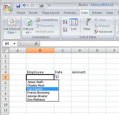
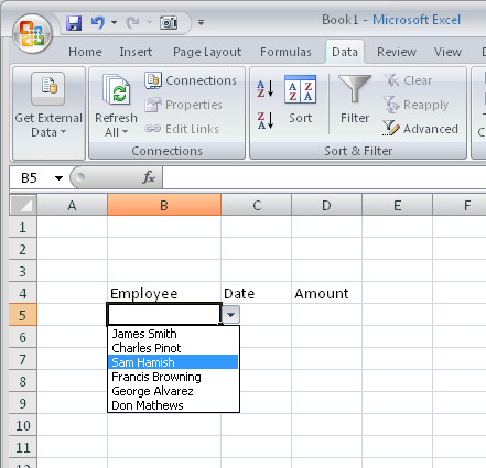
When you need to enter data from a small subset of entries into a range in Excel 2007 you can do it more easily using a custom designed dropdown list.
To configure a dropdown list in a cell type the list of items to use in a single column in a spare sheet in the workbook.
Select these cells and choose the Formulas tab Define Name, type DataForList as the name in the dialog, set the scope to Workbook and click Ok.
Switch to the sheet where you want to add your dropdown list to some cells, select the cells that should display a list of data to choose from and choose Data tab > Data Validation > Settings tab.
From the Allow: dropdown list choose List and, in the Source area, type =DataForList and click Ok.
Now, whenever you click a cell in this range you’ll see a dropdown list appear from which you can choose a list entry for that cell.
If you’re using Excel 2003, here is a link to an earlier post explaining how to do this in Excel 2003:
Automatic cell entries in Excel 2003
http://www.projectwoman.com/labels/validation.html
Helen Bradley
Labels: automatic, data entry, dropdown list, Excel 2003, Excel 2007
Categories:Uncategorized
posted by Helen Bradley @ 8:18 pmNo Comments links to this post