Thursday, July 23rd, 2009

Excel: Monthly totals for daily data


One issue I was faced with recently was the need to calculate monthly totals for worksheet data that was recorded for every day of the month for a few years.

I had a long series of dates with corresponding data in the cells to the right which I had downloaded from the web. The data needed to be viewed as monthly totals rather than as daily values for me to have a better picture of the changes over time.

The solution to doing this quickly and easily is a PivotTable. Here’s how to do it:

1
Select all the daily data including the column headings. If you have lots more columns of data than you plan to analyze, don’t worry, just select the lot for now.

2
In Excel 2007, choose Insert > Pivot Table. In the PivotTable Field List you now need to drag and drop fields into the respective boxes on the screen.

Drag the Date field into the Row Labels box and drag the field for the data that you want to analyze into the Sum Values box.

3
This gives you a list of dates and the data on the screen and you’re over half way to your monthly totals.

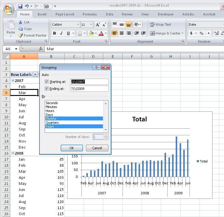
Click on one of the dates in the Row Labels column to select that cell, right-click and choose Group to display the Grouping box.

4
Click both the Month and the Years values in the list so that both are highlighted. Then click Ok.

5
Now your data will reappear grouped by the year and by the month within that year.

This allows you to analyze how the data has changed over time more easily than viewing it by day.

6
From here, to chart your data, click somewhere in the PivotTable, choose Insert > and then from the Chart area on the Ribbon click the Column option to create a column charts.

Select the chart sub-type and you’ll create a chart displaying the monthly totals from the PivotTable.

A PivotTable, while a little harder to get a feel for creating than a typical Excel formula, is actually the quickest and easiest way to summarizing this type data.

Helen Bradley

Wednesday, January 14th, 2009

Custom formats in Excel


Ok, so here’s the scenario, you want to enter a value like 20Kg (or 44 lb) into an Excel cell. All goes well until you try to multiply the value. Instant disaster. Your number isn’t a number it’s a piece of text and you can’t multiply or add text. You can’t divide or minus text or find the 4th power of it either – you get the idea.. it’s basically a useless entry – pretty but useless.

SO, how do you format a cell so it displays the Kg after the number but so it still treats the entry as a number? I’m so glad you asked!

The answer is to create a custom number format. Click the cell or a range of cells and choose Format > Cells > Number tab. Select the Custom entry and type something like 00.00 “kg” in the text box and click Ok. Now, enter the numbers again as 20 or 40 etc and the kg will appear automatically after the number courtesy of the format – and the number, well it’s still a number so you can add, multiply, divide and do all sorts of other wonderful things to it as you like.

You can also add the text before a number. So, for all those lovely Canada dollars I get paid by the folk at Hub Digital Living where I write a monthly Office column, I type a Custom format like “CAN” 00.00 in my sheet where I record my payments. It’s all so easly when you know how.. and now – you do too..

Helen Bradley

Saturday, January 10th, 2009

Converting Imported data in Excel

I encountered an interesting problem with Excel this morning when I tried to import data copied from a table in a PDF file. The table was bad news from my accountant about my retirement investments. I won’t be retiring any time soon 😉

The point of the issue however was that the data when copied and pasted into Excel came in neatly aligned in column but the numbers wouldn’t add up because they’d been added as text.

The solution to this is to use a feature previously called data parsing. What it does is to look at the data and convert it from one format to another. My only alternative would have been to select each cell, double-click on the cell to get the number on the screen, remove any characters that were causing issues such as any leading dollar signs or spaces and then press Enter to convert the text value into a number.

Luckily data parse does the work for you almost instantly. To do this, select the column of numbers that you’re working on. If you have a whole lot of columns to do, you still have to do each column one at a time. That’s the bad news; the rest of it is all good.

Select the column of numbers (if it includes some text entries that doesn’t matter), choose Data > Text to Columns and then select Delimited as the Original Data Type and click Next.

Click Next again and this is where you get to do the work. To convert text to numbers select the General option. If you have dates then select the Date option and select the date format that the data was created in. My values came from Australia so the date format used was dd-mmm-yy. Provided you select the date format that matches the dates you have, everything will convert just fine. Later if you want to show these in another format such as mm-dd-yy you do so using a date format. When you’re done, just click Finish.

The data will be instantly converted and you can move forward to do the same thing on the next column.

I estimate that this process took me about three minutes to do and on the data that I had it could have taken me half an hour or more to fix it all manually.

So next time you’ve imported data from an external source and when you need to convert text back into numbers check out the Data > Text in Columns option.

Helen Bradley

Friday, August 15th, 2008

Excel – Multiply cell values inside the cell


This is totally cool. I had no idea you could do it but I just tripped over this Excel feature.

Scenario: you have a list of values in a column that you want to multiply by a second value. Type the multiplier in a cell, anywhere. Click the cell and choose Edit > Copy so it’s on the Clipboard.

Now select the cells that contain the values you need to multiply. Choose Edit > Paste Special and click Multiply and click Values and click Ok. Excel replaces the values in the selected cells with the result of multiplying the values by the constant. It’s all done in situ so you don’t have to create new columns, multiply then paste the values back.

Oh, and there are options for Add, Subtract and Divide too so you can do all your math inside the current cell. Gotta love that!

Helen Bradley

Wednesday, April 30th, 2008

Sorting data in Excel

Sometimes the data in your worksheet doesn’t appear in the order you want it to. You can reorder the data by sorting it.

To sort data in a worksheet, select it using your mouse, or click inside the data area and press Control + Shift + * to select all the cells in the current block. In Excel 2003, choose Data, Sort and then choose the column which contains the data to sort from the Sort by: dropdown list. To sort on more than one column choose the second column from the dialog’s Then by: dropdown list. For example to produce a ‘phonebook’ type of sort, first Sort by the column containing the last name and Then by: the column containing the first name. If you do this, two people with the same last name will be grouped together but appear in alphabetical order by first name.

You can also sort in order of a custom list. So, for example, if you wanted all the people who live in Victoria to appear at the top of a list then those who live in NSW, etc.. create a custom list with the state names (or abbreviations) in the order you want to use for sorting. Then choose the State column in your data list as the Sort by: column and click Options. From the First key sort order dropdown list choose the custom list containing the state details and click Ok, and Ok again. The list will be sorted in order of the entries in your custom list and any entries which don’t match an item in the list will appear at the end, in alphabetical order.

Helen Bradley

Friday, March 21st, 2008

What’s in a name? Auto_Open or AutoOpen

Sometimes you wonder if the folks up at Redmond are laughing at us behind our backs. Really, do they deliberately set out to confuse us or are they just that plain disorganised?

Today my quandary involves Auto_Open and AutoOpen. These are two special macro names. The first, Auto_Open is Excel’s special named macro that runs automatically when the workbook containing it is opened. AutoOpen is the Word equivalent. It makes no sense that one has an underscore and the other doesn’t – it just makes life for us VBA folk a little more confusing than it should be.

The other macros Auto_Close and AutoClose work the same way, Auto_Close is the Excel macro name – call a macro by this name and save it in your workbook and it will run whenever you close the workbook. In Word, the name is AutoClose.

To add to the confusion, PowerPoint doesn’t support either of the naming conventions, in fact, you can’t create auto running macros in PowerPoint the same way you do in Word and Excel. The workaround is cumbersome, you need to create a PowerPoint add-in that includes the Auto_Open subroutine. Load the Add-in and PowerPoint will run the code in Auto_Open it loads and ditto for subroutine called Auto_close – it runs when the add-in is unloaded – which happens automatically when you exit PowerPoint. Learn more about how to do this in this KnowledgeBase article.

Thanks Redmond, we are now officially confused!

Helen Bradley

Monday, February 25th, 2008

Leading zeros in Excel

This is a fun solution. You want to put a series of numbers in a range in Excel and you want them to have leading zeros. So you want, 001, 002, 003 etc. Problem is that Excel drops the zeros when you type them. It makes sense, leading zeros aren’t required and really don’t aid comprehension. However, for your own reasons, you want them.

Here’s how to do this:

Select the cells and choose Format > Cells > Number tab. Select Custom from the Categories list and in the box marked Type:, type this:

00#

This tells Excel that there must always be 3 digits showing which forces leading zeros to be displayed. It doesn’t do anything to the numbers so they are still numbers which is just as you would want it to be.

Helen Bradley

Page 4 of 41234