Tuesday, May 1st, 2007
Ok, grey is my favourite colour – it’s the colour of my old school uniform. I’m an Aussie and we still wear uniforms to school! Mine was grey serge in winter and grey cotton in summer, complete with hats and gloves. I kid you not and this is seriously OT and it uses Australian spelling so I’ll get back to what I was saying.
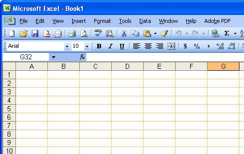
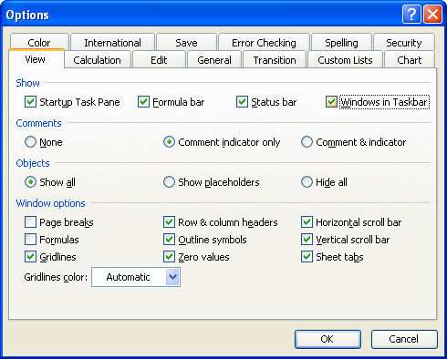
Ok, so gray might be my favorite color but it’s probably not yours. If Excel’s gray gridlines offend your color sense, you can change them or remove them entirely. To remove them choose Tool, Options, View tab and disable the Gridlines checkbox.
To change the color of the lines, choose Tool, Options, View tab and choose an alternate color from the Gridlines color dropdown list. If you didn’t realise gridlines were little dots and not solid lines, you’re about to see that that’s exactly what they are.
Helen Bradley
Labels: Excel 2003, gridlines
Categories:Uncategorized
posted by Helen Bradley @ 2:54 pmNo Comments links to this post
Tuesday, April 24th, 2007
There’s a special file in Excel called personal.xls which is opened automatically every time Excel opens. This makes it a great place to put your Excel macros as they’re then accessible to any open workbook.
Unfortunately, a personal.xls workbook is not created until you actually do it yourself so you may not have one. The simplest way to create one is to record a simple macro because then Excel does it for you.
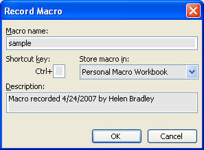
To do this, open Excel and choose Tools > Macro > Record New Macro and type a macro name. From the Store Macro In dropdown list choose Personal macro workbook and click Ok. Record a step or two—it doesn’t have to be an actual macro but it just has to be something and click the Stop Recording button or choose Tool > Macro > Stop Recording. Once you do this your personal.xls macro workbook will be created – ridiculously simple in fact.
If you’re prompted to save the file when you close Excel answer Yes to do so. Excel will save it in a location that ensures it will be opened automatically every time you open Excel. In future, store all macros that you want to be accessible to all workbooks in this file and you won’t ever have to load them specially.
Helen Bradley
Labels: Excel 2003, Personal Macro Workbook
Categories:Uncategorized
posted by Helen Bradley @ 3:43 pmNo Comments links to this post
Monday, April 23rd, 2007
Until I discovered how to add folders in the list down the left of the Word and other Office program’s Save As and File Open dialogs I spent hours navigating to get to the right folder to save a file. Some days it felt like it would be simply easier to dump everthing in the one folder and worry about finding it later on. Ok, I know – bad idea – but it was tempting.
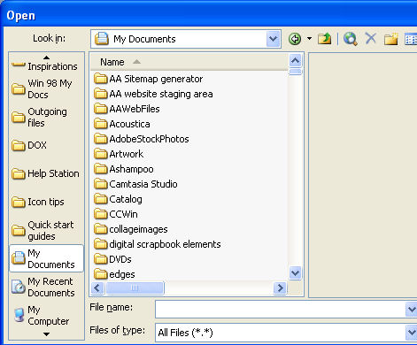
Now I fill my My Places list with all the folders I need long term and short term so saving files in the right folders is simplicity itself. All I do is click the folder in the list on the left and I’m there – just where I want to be.
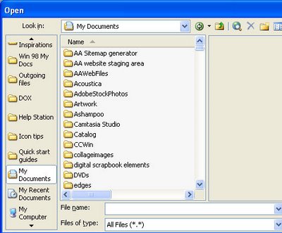
To do this yourself, from inside Excel or Word, for example, choose File, Save As and notice the My Places bar down the left of the Save As dialog. Navigate to the folder that you want to add to your My Places toolbar and select the folder. Click the Tools menu option in the top right of the dialog and choose Add to My Places. The folder will be automatically added to the bottom of your My Places bar. You can now click it to open the folder anytime you need it and it stays there from one Office session to the next.
Once you no longer need it, you can remove the folder from the list by right clicking it and choose Remove. You can also rename the folder and reorder items in the list by right clicking and choose Delete or Move Up/Move Down as required. You can also switch to small icons if there are too many folders in your My Places bar to see them clearly. The same folders turn up when you choose to open or save a file. Organization is just a click away.
Helen Bradley
Labels: Excel 2003, Microsoft Word, My Places., Office
Categories:Uncategorized
posted by Helen Bradley @ 3:24 pmNo Comments links to this post
Friday, April 20th, 2007
Sometimes it’s hard to get your point across in a text message because the nuances of your voice do not display.
When you’ve got something to say and you need it to be understood by someone viewing your worksheet, why not add a voice message rather than a text comment? It’s easy to do.
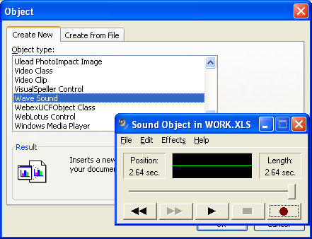
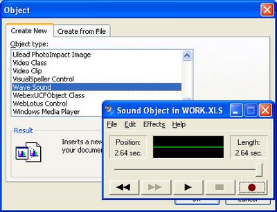
Choose Insert, Object and click the Create New tab. Click the Wave Sound option and the Window Sound object dialog opens. Click the Record button to record your message and when you are done click the Stop button.
A small sound object icon (it looks like a speaker) appears in your worksheet at the place that you were when you recorded the message – just click and drag it to where you want it to appear. It is saved with the file and can be played by double clicking on it.
Now you’ve got a better chance of people understanding exactly what it is that you’re trying to say to them when they hear you say it – well that’s the theory anyway!
Helen Bradley
Labels: Excel 2003, sound.
Categories:Uncategorized
posted by Helen Bradley @ 6:04 pmNo Comments links to this post
Thursday, April 12th, 2007
Sometimes you need to convert formulas into fixed figures – not often I admit, but often enough that there is an Excel tool for doing this.
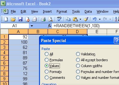
To convert any formula into a fixed value, select the cell or cells to fix and choose Edit > Copy and then immediately choose Edit > Paste Special > Values. Instantly your formulas are converted to fixed figures.
Helen Bradley
Labels: Excel 2003, paste special, values
Categories:Uncategorized
posted by Helen Bradley @ 8:03 pmNo Comments links to this post
Thursday, April 5th, 2007
Don’t you hate it when you know there’s something wrong but you can’t exactly put your finger on what is happening?
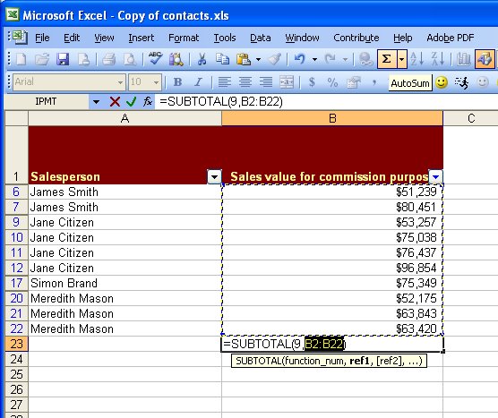
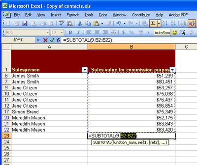
Try this, filter a list in Excel and write an =sum function at the foot of the list to sum the visible data. So far so good? Well, try checking that sum manually – do you still feel confident? Worse still, if you’re using Excel, try to filter the numbers in the column containing the Sum formula and watch as Excel chews up your formula – yikes!
You see, =SUM just doesn’t work on filtered lists. Instead, you have to use SUBTOTAL. Of course, there’s a simpler way. Use the AutoSum button on the Excel toolbar to create your formula and it does the sensible thing and writes a SUBTOTAL function for you. Now, when you filter the data it sums only visible values and it never gets swallowed up.
Helen Bradley
Labels: Excel 2003, filtered lists, sum
Categories:Uncategorized
posted by Helen Bradley @ 5:36 pmNo Comments links to this post
Sunday, April 1st, 2007

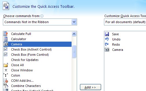
Did you know you can take a photo of an Excel range? Well you can and it’s one cool way to get around the problem of needing to print bits of two worksheets on the one piece of paper, something as smart as Excel is, it just can’t do.
To do this, right click a toolbar and choose Customize, Commands tab. From the Categories list choose Tools and from the Commands list click and drag the Camera icon up onto a toolbar. Now select a range on a worksheet and click the camera. Then click where the ‘photo’ should go.
Repeat this to assemble bits of lots of worksheets onto one page for printing. And the best bit? the photos are ‘live’ if the data in the worksheets changes, the photo does too!
Helen Bradley
Labels: camera, Excel 2003, range
Categories:Uncategorized
posted by Helen Bradley @ 10:11 pmNo Comments links to this post
Saturday, March 31st, 2007
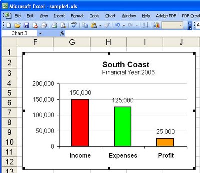
Data labels on your charts show your viewer the values they’re looking at and after all – isn’t that the purpose of the chart?
To add Data Labels to a chart, click the chart and choose Chart, Chart Options. Click the Data Labels tab and choose a style that will look good on your chart. Typically values is a good choice but, for pie charts, for example, a different type might work better.
Helen Bradley
Labels: chart, data labels, Excel 2003
Categories:Uncategorized
posted by Helen Bradley @ 9:54 pmNo Comments links to this post
Tuesday, March 27th, 2007

I like to see each individual worksheet I have open named on the taskbar – well, that is unless I don’t. When I have one of those “redecorating the desktop” days, I opt to have one indicator for Excel and then use the Windows menu or Control + F6 to switch between them.
Changing how I view my Excel interface is easy. Choose Tools, Options and click the View tab in the Options dialog. Disable the Windows in Taskbar checkbox to view one Excel indicator on the taskbar. Click Ok. Reverse the process to switch back.
Helen Bradley
Labels: Excel 2003, taskbar, window.
Categories:Uncategorized
posted by Helen Bradley @ 3:28 pmNo Comments links to this post
Friday, March 23rd, 2007
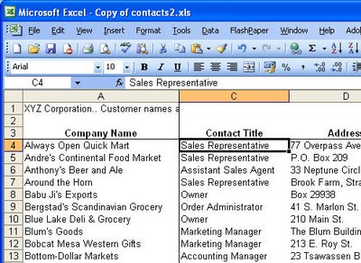
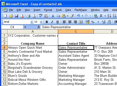
When you’re working on a very big spreadsheet it can get confusing as to what the headings are for the various rows and columns when you move away from the top most cells.
A simple way to solve this problem is to freeze panes – it’s a funny term for something that actually is very handy. Move so that cell A1 is located in the top left corner of your worksheet area and then position your cell pointer just below the set of headings that you want to see and just to the right of the column headings if they’re important too.
Choose Window, Freeze Panes and Excel will freeze the area above and to the left of where you are working. Now if you move around the worksheet wherever you happen to go the cells on the left and top of the worksheet will always be there.
If you need to undo the effect choose Window, Unfreeze Panes and it will all be back to rights. My guess is that you’ll like it so much that you won’t want to change it anyway.
Helen Bradley
Labels: Excel 2003, Freeze panes, window.
Categories:Uncategorized
posted by Helen Bradley @ 6:30 pmNo Comments links to this post