

When you’re working with different areas on an Excel worksheet it sometimes helps to name the area or range as Excel calls it.
You might do this so that you can easily select a print area from a number of different printing areas on the worksheet or where you want to move very quickly to a named area which is in an out of the way place on the worksheet.
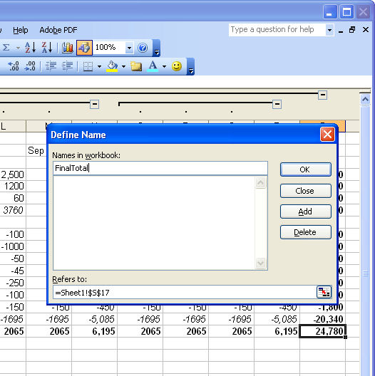
To name a range, select the cell or range of cells to name and choose Insert, Name, Define and give the cell or range a name. You can use whatever name you like, it just must be a single word name with no spaces and it can’t start with a number. When you’re done, click OK.
Now look up to the top left corner of the screen to the left of the formula bar you will see a small Name dropdown list. You can dropdown the list and select the named cell from the list and you will automatically go to it and, if it is a range, it will be automatically selected ready, for example, for printing.
Thursday, March 22nd, 2007
Pictures inside Excel comments
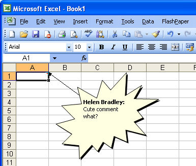
In a previous tip of the day, I showed you how to create shaped comments in Excel but today I’m going to go one step further and create pictures inside the comment.
As you might expect, start off in Excel and add a comment to a cell. Right-click the cell and choose Show comment and then click the border of the comment to select it. Choose Format, Comment and, from the Colors & Lines tab’s Color dropdown list choose Fill Effects and then the Picture tab and click Select Picture.
Find a picture to add to your comment from those in your My Pictures folder, enable the Lock Picture Aspect Ratio checkbox and click OK twice. You’ll now have the image inside your comment.
Depending on the image that you have used you may want to change the format of the text, for example coloring it a different color and sizing it large enough so that it can be easily seen.
For more tips and tricks and helpful Office columns, visit Projectwoman.com
Helen Bradley
Labels: comments, Excel 2003, images
Categories:Uncategorized
posted by Helen Bradley @ 6:27 pmNo Comments links to this post