Saturday, September 13th, 2014

Despite their existence in earlier versions of Photoshop some categories of filters are mysteriously missing from the menus in Photoshop CS6, Photoshop CC and Photoshop CC 2014. This is the default behavior so you won’t find the Artistic, Brush Strokes, Sketch, Stylize or Texture category of filters in the Filters menu. This is a problem if you use these filters so luckily you can bring the filters back when you know how.
It turns out that an option in the Preferences menu acts as gatekeeper for displaying the missing filter categories. To re-enable them, select Edit > Preferences > Plug-Ins…. Then check the box that reads Show all Filter Gallery groups and names. Click OK and restart Photoshop. This will put the filter categories back in the Filters menu.

Now you could have accessed the missing filters from the Filter Gallery but the way the filters are named in the Layers palette is different if you access them from the Filter Gallery rather than from the menu itself. So, if you use Convert for Smart Filters to create a smart object before applying the filters and if you start a filter from the menu then the filter name appears below the layer so you can tell the name of the filter you are applying. This image shows this situation:

If, on the other hand, you start your filter from the Filter Gallery the Layers palette simply shows Filter Gallery – with no indication of which filter you applied. This is what the Layers palette looks like – not very helpful at all.

In short, having the filters back on the menu and selecting them from there is the better option.
Be aware too that the Oil Paint filter was removed from Photoshop CC 2014 so it is gone for good.
Labels: categories, filter, filter gallery, filter menu, full, groups, Layers palette, list, missing filters, oil paint filter, photo, Photoshop, Photoshop CC, photoshop cc 2014, Photoshop CS6, restore
Categories:photoshop
posted by Hunter Delattre @ 10:00 amNo Comments links to this post
Thursday, June 12th, 2014
Free fonts for commercial use – thank you!
I’m making this post in celebration of the wonderful typographers who have made their fonts available for use in my projects. Creating an elegant and legible font can be very difficult; giving it away for free must be even harder. I would like to present some of my favorite fonts to help give them the exposure they deserve and pay the authors back for all of their hard work (and so you can enjoy them too!). These fonts are all free and take seconds to install. They’re also really really great.
Chalk Hand Lettering Shaded Font

Scrappy Looking Font

Cutie Patootie

Labels: favorite, fonts, free, list
Categories:photoshop
posted by Helen Bradley @ 10:00 amNo Comments links to this post
Monday, March 10th, 2014

Learn these quick techniques to format your Sticky Notes
I love using sticky notes to stick things to my desktop. Using these on my digital desktop is helping keep my real desktop clean and tidy. However, sometimes I need to format my notes and help for doing this is not easy to find. So, here, in a nutshell, are the super secret shortcut keys you can use to format your text on your sticky notes :
Bold                     Ctrl+B
Italic                   Ctrl+I
Underlined               Ctrl+U
Strikethrough            Ctrl+T
Bullet list              Ctrl+Shift+L
    (press this twice for a numbered list)
Subscript                Ctrl+=
Superscript              Ctrl+Shift++
Increase/Decrease font size
                        Ctrl+Shift+> and Ctrl+Shift+<
                        (or Ctrl+Scroll wheel)
Single space lines      Ctrl+1
Double space            Ctrl+2
1.5 Line spacing        Ctrl+5
Captialize Text         Ctrl+Shift+A
Right Align             Ctrl+R
Left Align              Ctrl+L
Center Align            Ctrl+E
You can also use fancy effects in sticky notes if you create them in another application such as Word and then copy and paste them into the Sticky Note.
Other handy Sticky Notes keyboard shortcuts:
Undo                    Ctrl+Z
Redo                    Ctrl+Y
Cut                     Ctrl+X
Copy                    Ctrl+C
Paste                   Ctrl+V
New Note Ctrl+N
To change the color of a note, right click it and choose a color.

To Backup your Sticky Notes:
You will find your Sticky notes file at
c:\users\<username>\AppData\Roaming\Microsoft\Sticky Notes
To make a backup, copy the stickynotes.snt file you find there.

To launch Sticky Notes if you haven’t yet discovered them:
Start > All Programs > Accessories > Sticky Notes
Helen Bradley
Labels: alignment, backup notes, change font, copy note, font size, format note, format sticky note, format text, list, sticky notes, stickynote, strikeout
Categories:Windows
posted by Helen Bradley @ 10:33 am4 Comments links to this post
Thursday, February 21st, 2013
Google Docs has the ability to use data validation to automate and manage data entry into cells in a spreadsheet. One way to do this is to limit the data that can be entered into a cell to a selection from a list that you create.
To see this at work, open an existing spreadsheet or create a new one. Select the cells into which the data will go and choose Data > Validation. From the Criteria dropdown list, select Items From a List and then click Enter List Items. Type each item for your list into the box separating entries from each other with a comma. Make sure the “Show list of items in a drop-down menu” is checked and if you don’t want a user to select anything that’s not in the list, then disable the “Allow invalid data, but show warning” checkbox. Click Save to save the validation options.

Now, when you enter data into any of the cells in the range you have configured this data validation rule for, you will see a dropdown indicator appear to the right of the cell. Click this and you can select an item from the list that is displayed below the cell. This data is entered into the cell in the same way as any data would be entered so you can, for example, use it in calculations by referring to the cell contents. In the example worksheet shown, a formula is used the cells in column C to calculate the converted value by checking what currency has been chosen and then multiplying the value in column A by the appropriate conversion rate.

It’s also possible to use other validation options using the Data Validation dialog. You can limit a cell entry to a number which meets certain criteria or to a text entry that contains or does not contain certain text or which is a valid email address or URL. You can also require that a date is entered within a certain range of dates or before or after another date.
You can force a user to comply with the data validation rules that you have created or allow them to enter an “invalid” value but warn them that they are about to enter data that doesn’t comply with the rule.
These data validation tools available in Google Docs are similar to those that you’ll find in other spreadsheet applications such as Excel.
Helen Bradley
Labels: data validation, google docs, items from a list, list, spreadsheet
Categories:hunter, office
posted by Hunter Delattre @ 9:00 amNo Comments links to this post
Tuesday, February 12th, 2013

Download a history of your Twitter Tweets today!
I could really do with a file of my tweets. It will help me to schedule future tweets by being able to recycle some of the best of our old ones. Luckily, recently, Twitter began offering this as an option. If you want to, you can download an entire file of your tweets from the first of them that you made.
To do this, log in to Twitter and go to your Settings, click Edit Profile and then click Account. Scroll to the bottom. There you will find a button Request Your Archive that you can press to get your tweets.

Wait and in a few hours and you’ll be emailed a link to download your entire archive.

This comes as a zip file which you must first unzip. There is an index.html file in the zip that you can run to view all your tweets in a browser interface. There are also other files containing them – such as a series of .csv files one for each month that you can open in Excel.

It’s a great way to get a permanent record of your tweets it you need it.
Helen Bradley
Labels: download, file, History, list, list of tweets, tweets., Twitter
Categories:General
posted by Helen Bradley @ 9:56 amNo Comments links to this post
Tuesday, May 4th, 2010

I don’t like Word’s basic bullet design and generally I’ll want bullets of my own liking. For example I’ll use bullet lists to create checkbox lists for things I need to do.
Bullet style
To get a checkbox list working in Word 2007 requires a little bit of list knowhow.If you’ve created your list items you can simply select the list and, from the Home tab, select the Multilevel list button and choose Define new list style.
You need to use this rather than the Bullet Lists > Define new bullet options because otherwise you don’t get control over the tabs and Word’s tab settings for bullets don’t always make good sense.
The Define New List Style option gives you the ability to control all of this. Start by typing a name for your list so that you can find it easily again later on. The select Bullets which is a small button to switch from numbers to bullet style. Click Insert symbol and select Wingdings as your font.
You can then select a bullet style such as a shadowed box, select it and click Ok.This is applied as the bullet style.
Spacing
To adjust the spacing between the edge of the page and the bullet and the bullet and the text, click the Format button and choose Numbering. Set the Aligned at value to the distance that you want between the left edge of the page and the bullet itself. I set this to 0 inches.
Set the text indent at a value to the distance you want between the bullet and the text. This is a hanging indent so it ensures that all lines of text are wrapped automatically to the value you set. I like to set this to .75 inches if I’m using large bullets. Click Ok. You can then click Ok again to set this as your bullet style.
You can ignore the rest of the numbering if you’re simply using a one level bullet. Click Ok.
To apply this bullet style to your document click the multilevel list and select the list style from the list styles area of the dialog. If you hold your mouse over it, you’ll see the list style appear in a small dialog with the name that you gave it showing. Click it to apply it to your list.
Helen Bradley
Labels: bullet list, Custom, list, list style, Word 2007
Categories:Uncategorized
posted by Helen Bradley @ 9:01 am4 Comments links to this post
Friday, October 23rd, 2009
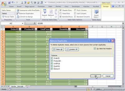
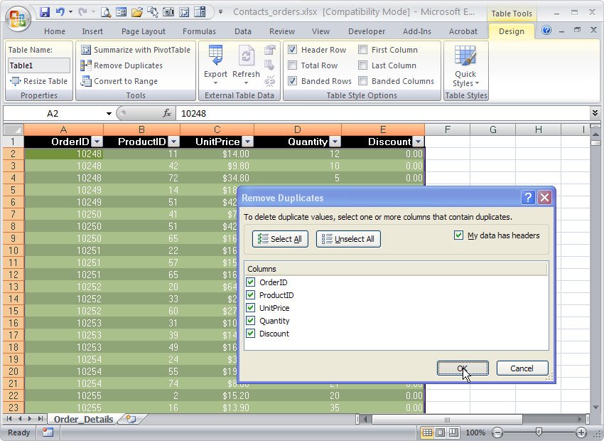
The new Excel 2007 has far superior tools for finding and removing duplicate entries in a list. Thankfully – because this has been a nightmare in earlier versions.
To find and remove duplicates from a list of data in Excel 2007 first format the area as a table by selecting it and, from the Home tab, choose Format as Table.
Click on any cell in the table and choose Table Tools > Design tab on the Ribbon.
Select Remove Duplicates to display the Remove Duplicates dialog. In this dialog are the Column headings for your data and all are selected by default. To remove the duplicate data from your worksheet leave all the column headings selected and click Ok.
If you want to remove rows where only certain data matches, leave the column headings for those particular rows selected and deselect the column headings for those columns which may have data that differs from one row to another. Now click Ok.
It is sensible to save your worksheet before running this Remove Duplicates option just in case you delete data by accident. If this happens and if you haven’t closed the file, you can recover it using the Undo button.
If you are using an earlier version of Excel, here are links to earlier relevant posts:
Excel – finding duplicates
http://www.projectwoman.com/2007/02/excel-finding-duplicates.html
Check for duplicates in an Excel list
http://www.projectwoman.com/2007/01/check-for-duplicates-in-excel-list-1.html
Helen Bradley
Labels: Excel 2007, list, remove duplicates, table
Categories:Uncategorized
posted by Helen Bradley @ 6:59 pmNo Comments links to this post
Thursday, August 13th, 2009
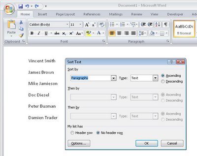
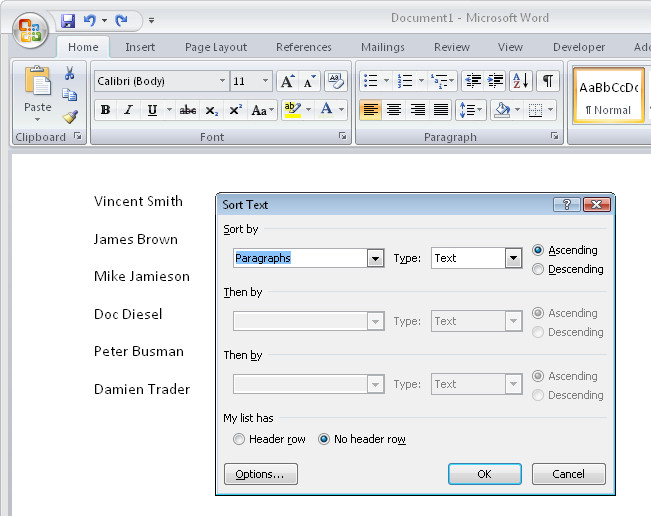
Word 2007 finally fixed a huge problem that existed in earlier versions – it looked like there was no way to sort data in a list.
This wasn’t the case – you used the table sort feature but it was far from being self evident.
Now Word 2007 uses the same tool it just puts it in a smart place.
To sort a list or series of words or paragraphs, select the text.
From the Ribbon, click the Home button and click the Sort button in the Paragraph group.
Choose Paragraph to sort on the first word and click Ok to sort the data in order.
If you’re using an earlier version of Word, then visit this post to see how to sort in Word 2003 and earlier:
Sorting a Word list
http://www.projectwoman.com/labels/Table%20Sort.html
Helen Bradley
Labels: list, Ribbon, sort, Sort button, Table Sort, Word 2007
Categories:Uncategorized
posted by Helen Bradley @ 7:23 pm2 Comments links to this post
Friday, February 16th, 2007
Excel 2003 offered a cool new tool for managing data that was in a list format. It made Excel the place of choice for small lists and it simplified the process of charting list data – Excel lists expanded automatically to allow for more data to be entered and charts based on the list data automatically expanded to include the new data – wonderful!
Here’s how to work with lists in Excel:
- Turn an existing table of data into a list by clicking on a cell in the range and choose Data, List, Create List. If your list has a heading row, enable the My list has headers checkbox and click Ok. Notice the border around the list.
- To add a row, click in the list area and click in the last (Insert) row which has an asterisk in its first cell. It is also possible to add a row in the middle of the list by clicking where the row should appear and choose List, Insert, Row.
- When data is created as a list, the AutoFilter feature is enabled. To sort data in the list, click the dropdown arrow to the right of the column (field) to sort on and choose Sort Ascending or Sort Descending as required. To sort on multiple columns, use the Data, Sort dialog.
- To create a complex filter for your list, click the Custom option from the dropdown list for the field that you want to create the query on. Set the tests to use and select And or Or depending on what information you need to extract. Click Ok to view the results. To display all records again, choose Data, Filter, Show All.
- When you create a chart based on list data it will be automatically updated when you add a new item to the list. To create your chart, click in the list and click the Chart Wizard button on the new List toolbar and proceed through the Wizard as you would for any other chart.
- To perform calculations on list data use the Toggle Total Row button. This adds a total row to the list and totals the right most column. To disable this total or create another one, click the down pointing arrow to the right of the total and choose None or a different calculation. Each column has its own down pointing arrow from which you can select the calculation to be made on that column’s data.
Helen Bradley
Labels: chart, Excel 2003, list, table data, total row.
Categories:Uncategorized
posted by Helen Bradley @ 7:22 pmNo Comments links to this post
Saturday, February 3rd, 2007
We all love to save time and here’s a great tip to make repetitive cell entries in Excel just so much easier to complete.
You do this by making a drop-down list in a cell so you can select your entry from it rather than having to type it fresh each time.
To do this:
- Type the list of items to use in a single column in a spare sheet in the workbook.
- Select these cells and choose Insert, Name, Define and type DataForList and click Ok.
- Move to the sheet where the data goes, select the cells for the drop-down list and choose Data, Validation, Settings tab. From the Allow list choose List and, in the Source area, type =DataForList and click Ok.
Now, whenever you click a cell in this range you’ll see a list box indicator appear and you can choose the cell entry from the list.
Helen Bradley
Labels: cell entry, define, Excel tip, insert, list, name, validation
Categories:Uncategorized
posted by Helen Bradley @ 9:02 pm1 Comment links to this post