

Thursday, July 5th, 2007
Multipage tables in Word
When you make really big tables in Word that span multiple pages you get into trouble when you try to read the text on the second and subsequent pages of the document because there are no table headings displayed.
Your gut reaction migth be to edit the table and to insert rows for the headings on each of the pages – good idea but there is a better one.
Select the rows at the top of the table that contain the headings – this might be one row or it could be a couple. Now choose Table, Heading Rows Repeat. Voila! Word does all the work for you – it puts the duplicate headings anywhere they need to be – if you add more text to the table or remove text – the headings are always in just the right place – much less effort and a much better end result.
Labels: heading rows repeat, Word table
Wednesday, July 4th, 2007
Boy was this annoying! HP Vista computers…
Ok, I just bought a new Vista tablet from HP. Let me start by saying it’s a great machine… but, here’s the rub, there is this very annoying popup that keeps appearing asking if you want to set up HP internet services. Well I would say yes if I hadn’t already done it so I click no and don’t ask me again and I get back to watching my Netflix Watch Now movie. Only a few minutes later, there it is again and again and again and again.. ad nauseum, every day every few minutes when I’m surfing the web already – talk about annoying and very stupid to boot.
Eventually I can see that saying Don’t ask me again is not going to work so I go looking for a solution. The solution is that this popup is running via a scheduled task. To stop it, log in as administrator if you aren’t already, open Control Panel and locate and find the Administrative Tools option. Locate Scheduled tasks and you’ll find the InternetServiceOffers option in the running tasks list which is what is causing the issues. Right click this option and disable it and, voila! no more stupid prompt and I can get back to my movie.
Happy 4th!
Wednesday, July 4th, 2007
Excel – highlight cells containing formulas
There’s no shortcut way to color code cells in Excel which contain formulas but this workaround is simple and fast.
Choose Edit, GoTo, Special button and click Formulas and then Ok. Now fill the cells with a color using the Fill Color tool.
It’s now clear which cells contain formulas and those that do not.
Monday, July 2nd, 2007
No new file when you launch Excel
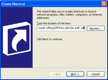
When you open Excel you will, by default see a new blank workbook. If you’d prefer to see nothing at all you can do so by altering the Excel startup icon.
Right click it and choose Properties and then in the Command area add the text /e at the end after the double quotes. Now Excel will launch without the splash screen and with no new workbook.
Labels: command line switch, Excel 2003, startup
Friday, June 29th, 2007
Fixing misspellings – Word
It happens just when you don’t want it to – you press the wrong key and all of a sudden you’ve saved an incorrectly spelled word to your dictionary. Unless you fix the problem, Word won’t pick up this misspelling ever again.
To solve the problem, choose Tools, Options, Spelling & Grammar and click the Custom Dictionaries button, click Custom.dic and click Modify. Locate the misspelled word, select it and click Delete.
Now click Ok and you’re done.
Labels: dictionary, misspelled words, Word 2003
Wednesday, June 27th, 2007
Word – Quick and easy columns…
One thing I do amongst all the things I do is to tech edit articles and books.
You learn a lot when you do this, on the one hand you learn how much you don’t know and on the other you learn how much you do know… it’s an eye opening experience both ways.
One thing that came out of a recent experience is how to do columns in Word. In this case, I liked my solution lots better than the one in front of me.
To turn a piece of text you have already created into a series of columns in Word, select the text and choose Format, Columns. Now choose how many and the width of your columns and instantly – columns to go!
I won’t disclose the solution I was editing… it simply wasn’t this simple.
Wednesday, June 27th, 2007
Gridlines – Yes or No?
In Excel there are gridlines and gridlines. You can display them on the screen as you work or on the printouts or both or neither.
Confusing?
To display or hide gridlines as you work, choose Tools, Options, View tab and enable or disable Gridlines.
For printing, choose File, Page Setup, Sheet tab and enable or disable Gridlines for printing…
Now you know.
Labels: Excel 2003, gridlines
Tuesday, June 26th, 2007
Word – Click to type blocks
The MacroButton field code in Word is handy for creating “Click Here” blocks in your documents indicating what needs to be typed and where. When you use these blocks, you simply click and type the entry required.
To create a click here block, choose Insert, Field, from the Categories list choose Document Automation and from the Field names list choose MacroButton. In the text area, after the word MACROBUTTON, type:
NoMacro [Click here and type a name]
Click Ok to finish. Provided you’re displaying field code results and not the codes themselves, you’ll should see the prompt text appear inside the square brackets. Save your document. Then, when you open and use the document you can complete the required text by clicking the prompt and type the requested data. Notice when you do this that the field code text disappears and is replaced by your text.
Labels: click to type block., Word
Friday, June 22nd, 2007
Excel Pasting column widths
Copy and paste a range in Excel and you get everything except the column widths. They get left behind and sometimes that’s a big nuisance. When you need to paste column widths too, paste your cells and don’t move. Choose Edit, Paste Special and click Column widths and the column widths of the new cells adjust to match the source.
Easy when you know how…
Labels: column widths., Excel tip
Thursday, June 21st, 2007
Versioning in Word
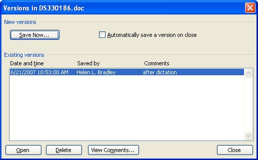
Ever had that “Woops! I shouldn’t have deleted that!” feeling? If you use versions in Word, you never will. Versions let you save a copy of the document’s current status in the document file. Each new version is stored in the same file so you can return to a previous ‘version’ any time.
To save a version and configure it to happen automatically, choose File, Versions and click Save Now. You can also configure it so a version for your file is saved each time the file is closed. Then, using the same tool you can view and use an older version of the file whenever you need it.
If you’re prone to changing your mind, it could be just the tool you need!
However a word of warning, versioning isn’t supported in Word 2007 and you’ll lose your versions if you open and save a versioned document using Word 2007. So, this tool is only for those of you who haven’t yet upgraded.
Wednesday, June 20th, 2007
Millions in Excel
Excel has some cool formatting tricks up its sleeve and one of these is its ability to shrink really big numbers down to size.
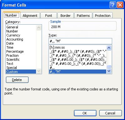
So, if you have values in the millions – like your salary – Ha!, you can size them down to size using a custom format. Select the cells, choose Format, Cells, Number tab and click the Custom group and type #,,”M” and Excel will format 200,000,000 to read 200M! The numbers aren’t altered it’s just a simpler way of displaying them.
Since the Y axis of a chart inherits its formatting from the top left cell in the chart data range this lets you format a chart’s Y axis to show the smaller values too.
Labels: Excel 2003, Excel 2007, number format
Tuesday, June 19th, 2007
Outlook Notes anywhere
Still on the subject of Outlook Notes (on the basis of when you’re on a good thing stick to it), did you know Notes can be dragged out of Outlook?
Go ahead, grab a Note adn drag it out of Outlook. Put it anywhere you like – it will sit on the Desktop or your Quick Launch bar. If you close Outlook, you can view the note’s contents without having to open Outlook by just double clicking on it.
This feature makes an Outlook Note something of much higher value than before. Need to remember a phone number? Type it into a Note and drag and drop it to your Quick Launch bar and it’s there handy for when you need it.
Labels: notes, Outlook 2003, Outlook 2007
Monday, June 18th, 2007
Color Your World – Outlook Notes
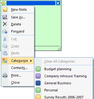
Ok, so yellow sticky notes just don’t work for me. I’d rather mine were, well, anything but yellow. In Outlook 2007 you can color your Notes by clicking the indicator in the top left corner, choose Categories and then the category to assign the note to – the category color becomes the Note color. In Outlook 2003, click the indicator in the top left corner of the note and choose Color and then a different color for your note.
To change the default color in Outlook 2003 and Outlook 2007, choose Tools, Options, Preferences tab and click Note Options. Set the Color value to your chosen color and click Ok twice. There’s only a limited color selection available this way but it does make a change from yellow.
Labels: default color, notes, Outlook 2003, Outlook 2007
Saturday, June 16th, 2007
Self Portrait in Excel
Excel can take photos of itself, it’s a fun technique for applying a portion of a worksheet back into the worksheet as an image or into some other application.
To do this, make a selection around the area you’re interested in and hold Shift as you click to open the Edit menu. There’s a new option called Copy Picture which, if you click it, you can then select how to copy the picture – as shown on the screen or when printed etc.. Make your choice and then you can paste the image into any application.
To paste it back into an Excel workbook, Shift + click on the Edit menu and you can paste it back in by choosing Paste Picture.
You can do some funky things with this. Take a copy of a portion of a worksheet using this technique and then select a bar in a bar chart. Choose Edit, Paste and you’ll paste the image in as your new bar chart fill.
Labels: chart image, Excel 2003, take a picture of a worksheet
Thursday, June 14th, 2007
A map to find your way around – Word
The Document map tool in Word is a cool way to find your way around a long document. Click the Document Map icon on the toolbar in Word 2003 or earlier or choose View, Document Map and it appears down the left of the page. In Word 2007, the Document Map checkbox is on the View ribbon tab.
If you use styles, in particular the heading styles, the items formatted with these styles appear in the list. Simply click one to move automatically to that item.
It’s simple and a smart way to find your way around a seriously big document.
Labels: document map., Word 2003, Word 2007