Wednesday, April 18th, 2012
Unhide Hidden PowerPoint 2010 animations
Sometimes when you’re working in PowerPoint you’ll notice that an animation is not available and it is greyed out.
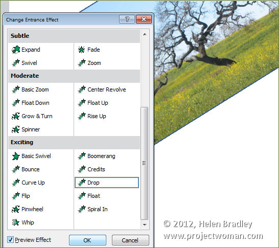
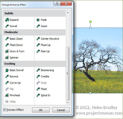
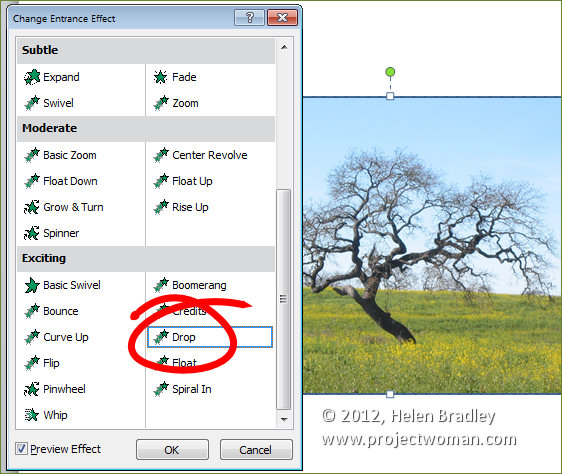
For example add an image to a slide and then try to select the drop animation from the Entrance Effects. It’s not available because what you’re trying to select is a tool that is used to animate text and you are using an image.
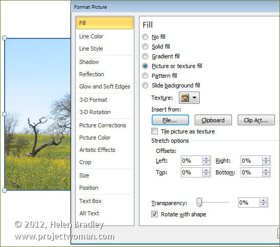
However you can use this animation on an image, you just need to know how to do so. To do this, place the image inside a shape. So, add a shape to the slide – a plain rectangle will do, and as the shape background add the picture by right-clicking the shape, choose Format Shape and then from the shape Fill options select Picture and fill it with a picture.
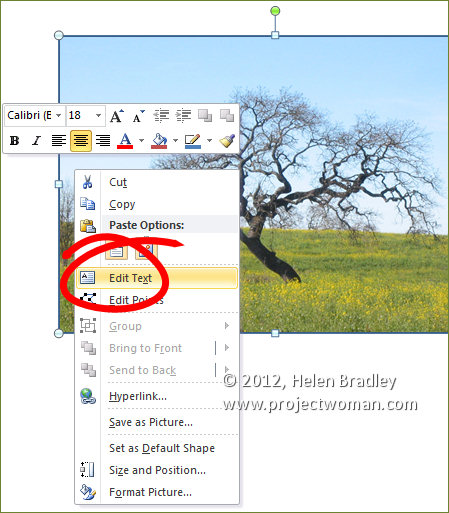
Right click the shape and choose Edit Text and press the spacebar a couple of times so that you add some text to the shape – spaces won’t show but they are text. It’s critical that you do this because without the text the shape will not be able to be animated using text animation tools.
Now when you select the Animate options and the Entrance Effects you’ll find that the effects that you couldn’t use before like Drop, Flip and Whip are now available because you’re working with PowerPoint deems to be a text object.
Labels: amimation pane, animate, animations, drop, entrance effects, flip, grayed out, greyed out, Helen Bradley, hidden animations, PowerPoint, PowerPoint 2010, timeline, whip
Tuesday, February 21st, 2012
Excel – conditional sums
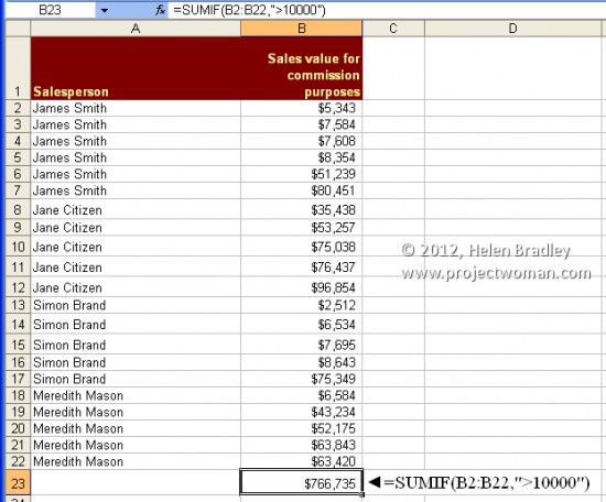
In some instances you may want to sum a column of numbers depending on the contents of that column. For example, if you want to total the sales figures in the range B3:B35 but only where those values are greater than 10000, this SUMIF formula will do the work:
=SUMIF(B3:B35,”>10000″)
The Sumif function takes first the range to sum and then the condition to match. In this case you will be summing all values in column B from rows 3 to 35 inclusive which contain values greater than 10000.
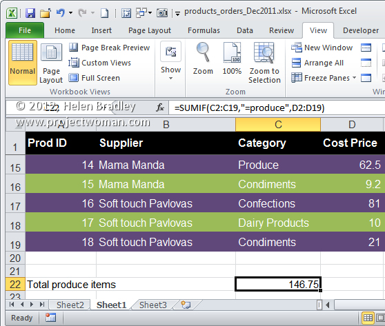
The SUMIF function can also sum a different range than that used for the test. Here it sums all values in the range D2:D19 where the corresponding values in the range C2:C19 are Produce.
=SUMIF(C2:C19,”=produce”,D2:D19)
Labels: conditional sum, Excel 2010, sumif
Sunday, February 19th, 2012
DIY Excel functions
With a little bit of coding experience it is possible to create your own functions in Excel 2010 and earlier.
In Excel 2010, make sure the Developer toolbar is visible – if it is not, follow this post to make it so.
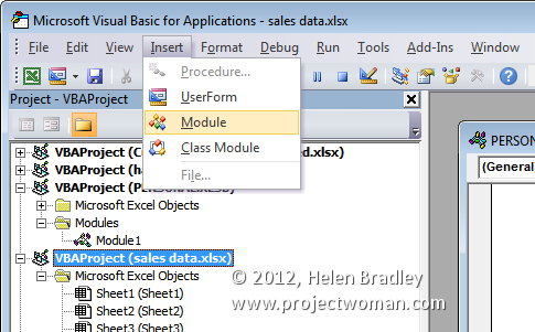
Now choose Developer tab and click the Visual Basic button. In the Project – VBAProject pane, select the current file and choose Insert > Module.
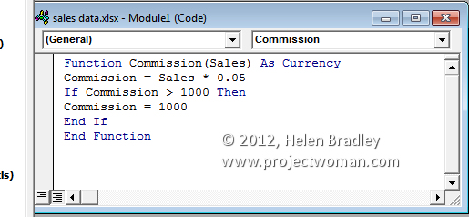
Type this function into the dialog and then close the VB editor and return to your worksheet:
Function Commission(Sales) As Currency
Commission = Sales * 0.05
If Commission > 1000 Then
Commission = 1000
End If
End Function
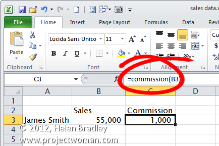
To test your function type this formula into a worksheet:
=COMMISSION(20000)
or as shown here:
=COMMISSION(B3)
The function calculates commission at 5% of the amount of sales. If the 5% value is more than $1,000 then the commission is pegged at this amount – to check this, test the function with a very large number. Functions created this way are only able to be used in the current workbook.
Labels: calculate commissions, diy functions, Excel custom functions, Macro, vb editor, vba code
Tuesday, January 10th, 2012
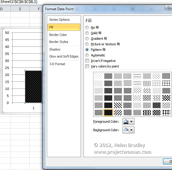
Pattern fills for your Excel 2007 charts
In Excel 2003 and now in Excel 2010 , there are pattern fills which you can use to fill chart bars so your charts print just great in black and white.
Unfortunately the same feature was removed from Excel 2007 – wtf? I have no clue why but it was but it has to be a very silly thing to have done.
If you are using Excel 2007 and you need to use pattern fills with a chart you are out of luck – well not really – you just need to read the rest of this tip because I can tell you how to put the fills back into Excel 2007.
To begin, download this handy add-in: http://officeblogs.net/excel/PatternUI.zip
Update: This link is no longer live so patternui.zip is not longer available. You can find an add-in here (with instructions which achieves the same thing) courtesy of Andy Pope.
The zip file contains a single file patternUI.xlam which you need to extract and place somewhere you will find it easily and where it won’t get deleted by accident. You could make an Excel add-ins folder for it, for example.
Once you’ve done this, open Excel 2007 and choose the Office button > Excel Options > Add-ins and from the Manage dropdown list, select Excel Add-ins and click Go. This opens the old Add-ins dialog from earlier versions of Excel. Click Browse and locate the .xlam file that you just unzipped and placed somewhere safe. Select it and click Ok. Ensure that the PatternUI option appears in the Add-ins available list and that it is checked and click Ok.
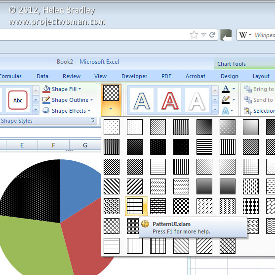
Now create an Excel chart. Once you have you chart, click on the data series to fill with a pattern – if you have a single series plotted then select just one of the columns at a time. Select the Chart Tools > Format tab and notice that you now have an option called Patterns available. Click the Patterns option and select a pattern to apply to the currently selected chart series or column. Click on each series or column in turn and apply a pattern to it. When you are done, you can print your chart as usual.
Installed add-ins are managed automatically by Excel so you will find that the add-in will still be there and accessible next time you use Excel.
If you are using Excel 2010 you don’t need this add-in as the pattern fills are back where they should have been all the time.
Labels: add-in, black and white, charts, download, Excel 2007, Excel 2010, free, pattern fills
Wednesday, December 28th, 2011
Quickly access Excel 2010 formula requirements
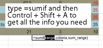
Ok.. so you want to use an Excel formula and you know it is, say, SUMIF that you want to use, but what data does it need and where?
Before you go searching through help or cranking up your browser, let Excel do the work for you. Just type =SUMIF in a cell and press Control + Shift + A and Excel will give you the list of data required. It’s dead simple and it saves heaps of time.
Labels: arguments, Excel 2010, formula, function, quick find
Thursday, November 17th, 2011
Save space – Compress your images in Word
A reader just asked if they added 50 images to a Word file would that blow out the file size when they send it to their colleagues. Answer: Yep! big time.
Most specially if you use your your beaut iPhone to capture the images, or a good compact camera or if you just insert big pictures. You see, unless you do something those big pictures will be inserted in the file and included in it when you save it – you can end up with a monster Word file (think 5Mb x 50!)
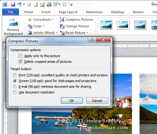
The solution to the problem is to compress the images. To compress all the images in your Word 2010/2007 file so that they take less room, click on any image and choose Picture Tools > Format tab. Locate the Compress Pictures button and deselect Apply only to this Picture so all images will be compressed.
If there is an Options button click it to see the sizing options (this appears in Word 2007 but not in Word 2010). Then choose the Target output – typically Screen or Print are good options as they will view well and print just fine. Check the Delete Cropped Areas of Pictures checkbox so cropped data won’t be saved. Click Ok. Then save the document.
This compression feature will reduce your file to a better size for sharing without compromising the quality of the document. And the changes affect only the images in the document not the originals on your disk.
Labels: compress images, Picture, reduce file size, reduce size of files, shrink, squash, Word 2003, Word 2007, Word 2010
Tuesday, October 18th, 2011
How to set up your PC and your iPad for the free iWork and iCloud
If you have an iPad and if you have upgraded to the new iOS 5 then you can take advantage of the free iCloud and iWork tools for synching files and storing them in the Cloud. iCloud allows you to synch not only photos but also data such as files across your devices. So you can use this new technology to share Microsoft Office documents with Numbers, Keynote and Pages on your iPad. And you do this on your PC using a browser and by passing iTunes – something I for one am really glad about.
So, if you’re using a Windows PC, you can automatically access documents that have been sent from the iPad to the iCloud without needing to plug your iPad into your computer or use iTunes. It is a long over due technology and it provides a more professional approach to the task of file exchange – not to mention it will solve the problem that some users experience where their network administrators block iTunes.
Getting this all configured is simple but it is far from intuitive. Nowhere could I find step by step instructions so I had to piece this stuff together bit by bit. Hence this post – it will explain all you need to do. From start to finish, I’d allow about 1.5 hours – if you finish early that’s a bonus but none of this stuff is totally trivial so allow time to get it all done.
Start by updating iTunes to 10.5 on your PC. If you haven’t done this – you do this from inside iTunes. Then, connect your iPad to your PC and update the iPad to iOS 5 – this might take some time depending on how much data you have on your iPad as everything will be backed up – then reinstalled once the operating system is updated.
While iTunes is updating and iOS 5 is being configured, you can – on your PC – visit the Apple site at http://support.apple.com/kb/DL1455 and download and install the iCloud control panel for Windows.
Back on your iPad when everything is running again, go into Settings and create your iCloud account.
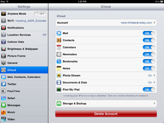
On the iPad, in Settings > iCloud you can set up syncing for email and other items such as your Photo Stream and Documents & Data. For Documents & Data you have a choice of using your cellular data plan to upload or Wi-Fi only – for your Photo Stream you can only synch this using Wi-Fi.
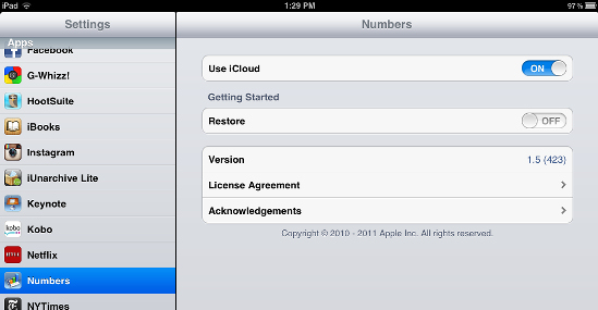
If you have Numbers, Pages and/or Keynote installed, in Settings select these each in turn and enable the Use iCloud option – you need to turn this On before any of these apps will access iCloud.
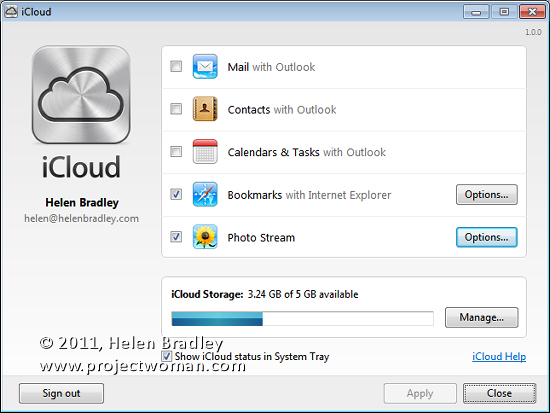
iCloud can be accessed on your PC by opening the system tray and clicking on its icon – if it isn’t there, choose the Start menu and type iCloud. Use the settings to configure how and what you want your iCloud and iPad to share. For example, click Photo Stream and configure a folder for images to upload to the iPad and one to use to download into. On the PC you can select whether email, contacts and Calendars & Tasks should be shared with Outlook. I suggest you backup your Outlook pst file before you even consider enabling this!
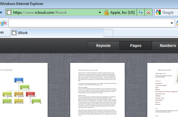
So far you have everything working except your documents. For this, confusingly enough, you head back to your PC and crank up your browser and visit www.icloud.com. Sign in using your Apple ID. If prompted you should download and install the browser plug-in.
Here you will find links for Keynote, Numbers and Pages. Click on one of them to view the documents synched from your iPad – first time you do this it might take a while as the synching takes place.
In future, every time you create a document on your iPad or edit one it will be synched automatically and will appear in this list.
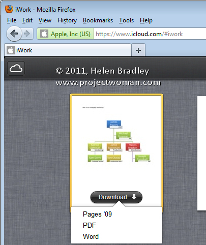
Although it is not obvious that you can do this, you can also drag and drop a document, spreadsheet or PowerPoint document into the appropriate panel and it will be synched with your iPad. You can double click a document in the list to download it to the appropriate application on your computer – here I’ve chosen a Pages document which will open in Word.
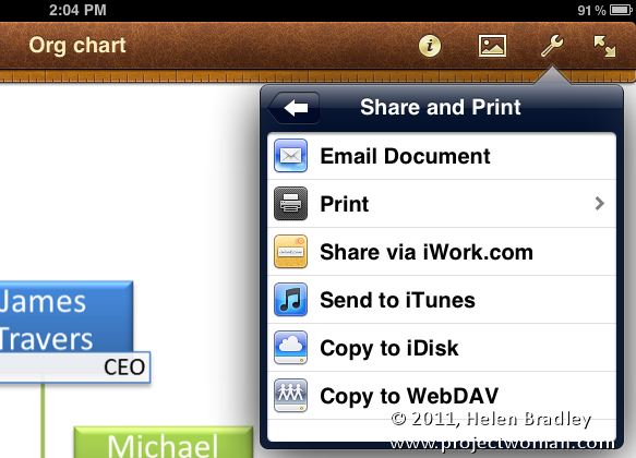
You can also now share documents with others who have Apple IDs using iWork. So, on your iPad, open a document, spreadsheet or presentation and click Share and Print (it looks like a spanner) and choose Share via iWork.com. Type the email address of the person you want to share it with and they will receive an invitation to view the shared document:
Labels: cloud sharing files, excel cloud, file sharing, free apps, free iwork, icloud, ios 5, ios5, itunes 10.5, iwork, keynote, MSWord cloud, numbers, pages, powerpoint cloud
Monday, October 17th, 2011
Shape images and Clip Art in Word 2010
There is a healthy range of free clip art available from Microsoft and it includes some photos including content from iStockPhoto.com. However, the process of getting them into your document any other way than by choosing Insert > Clip Art is not always obvious.
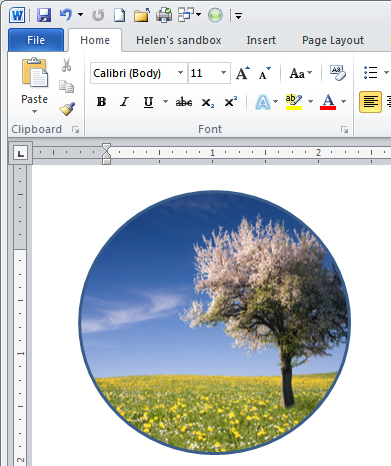
Here’s how to add a clip art image to a circle shape:
Choose Insert > Shape and select the Oval. Hold Shift as you draw to create a circle on the screen. If you choose Drawing Tools > Format > Shape Fill you get the option of applying a picture to the shape but not clip art.
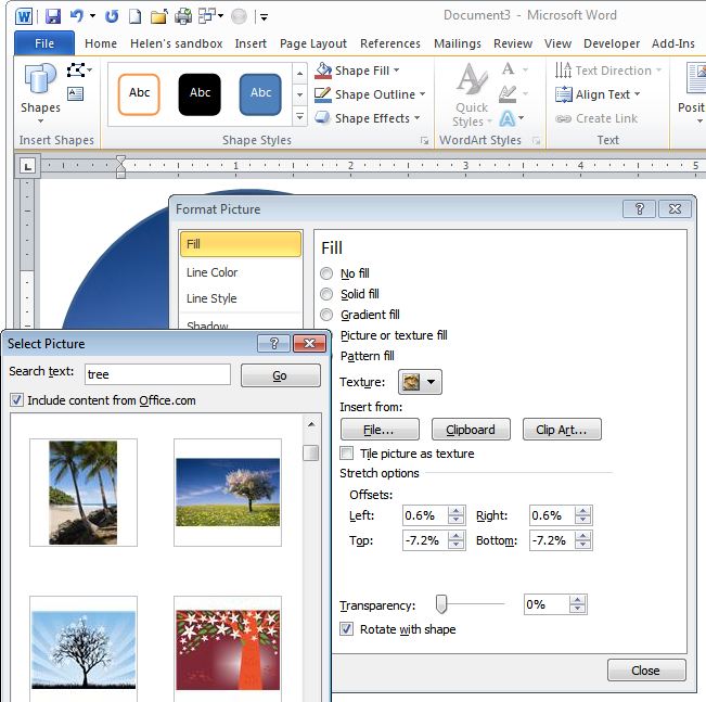
Instead, right click the shape and choose Format Shape to get access to the new to Word 2010 – Format Shape dialog. Choose Fill > Picture or Texture Fill and click the Clip Art button.
Browse or search for an image. You could also have placed a Clip Art image into your document using Insert > Clip Art and then selected it and cut it to the Clipboard. Here in this dialog you can choose Clipboard to add the image from the clipboard – in short you have more options here for using image than you have using the Shape Fill list.
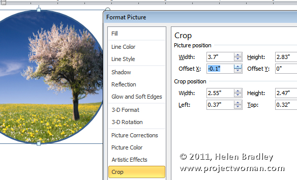
If the image is skewed out of shape – and it will be if it is a portrait or landscape image inside a circle which is pretty much a square with the corners cut off – you can adjust it.
Select Crop and, for a landscape orientation image inside a circle, increase the Picture Position Width value. For a portrait orientation image inside a circle, increase the Picture Position: Height value.
Then adjust the Offset X or Offset Y values, if desired, to control which portion of the image shows up inside the circle.
Labels: clip art, images, Microsoft Word 2010, photos, pictures in shapes, shapes, Word 2010
Friday, October 14th, 2011
Reformatting pasted text in Word
I recently grabbed some text from an email that I’d sent to someone. The text was in numbered point form and I wanted to add some more items inside the list of points. This is where everything started to go hair-raisingly wrong.
It seemed as if my list was no longer reformatting correctly and the numbers were everywhere. Worse still, that old standby of copying and pasting formats using the FormatPainter didn’t fix the problem.
By selecting the Show/Hide¶ icon on the Home tab in Word I immediately saw the problem. Instead of paragraph marks at the end of each paragraph there were bent arrows indicating a manual line break. I didn’t put them there but the email software had.
To get my list back to something that I could work with, I needed to quickly replace the manual line breaks with paragraph breaks.
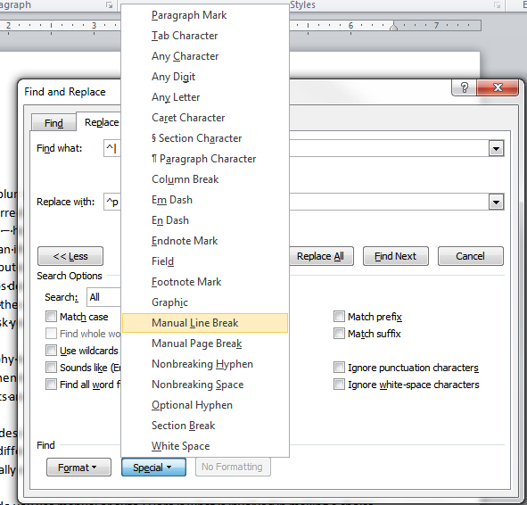
If you open the Find and Replace dialog and click in the Find What: box you immediately see the problem – how do I tell it what a manual line break is and what a paragraph break is? The solution is to click the More button to show more options. Then click Special to get access to the Manual Line Break character. It’s actually a carat and what looks like a pipe symbol but it’s easiest to get this by clicking this by clicking Manual Line Break because the pipe symbol on the keyboard isn’t the right one – go figure!
Then click in the Replace With box and select the Paragraph Mark – this one you can type manually as it is carat + p (^p) but since you’re there why not click to insert it instead. Now click Less to return the dialog to what it looked like before and click Replace All to turn all the manual line breaks back to regular paragraph marks. Now my numbering worked just fine.
Labels: find and replace, manual line break, paragraph marker, special characters, Word
Wednesday, October 12th, 2011
Excel – get the day or month name from a date
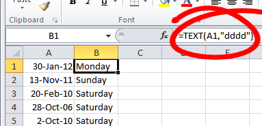
Often you will want to extract a month or day of the week from an Excel date. This is extraordinarily easy to do using the text function.
To get the name of the day of the week from a date in, for example, cell A1 type this into another cell:
= TEXT(A1,”dddd”)
This will give you the full day name spelled out such as Monday or Tuesday.
If you want a three character name use:
= TEXT(A1,”ddd”)
The same basic formula can be used to get the month of the year from a date. Use this to get the month name spelled out in full:
= TEXT(A1,”mmmm”)
Use this to get the month of the year spelled out in three characters:
= TEXT(A1,”mmm”)
and this for a single letter month:
= TEXT(A1,”mmmmm”)
This formula can be easily constructed and copied down a column of dates to extract just the information you want very quickly and easily.
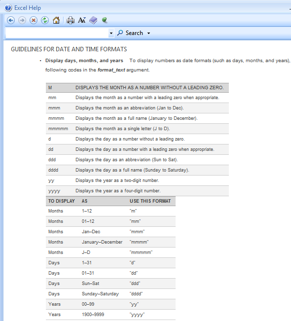
The Excel help file has some information about the different formats you can use to extract data using the TEXT function.
Labels: day of the week from a date, Excel 2007, Excel 2010, functions, month name from a date
Monday, October 3rd, 2011
Go To a cell in a formula in Excel
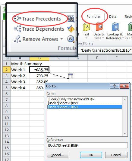
Consider this scenario – you have a cell which contains a link to data in another cell on another sheet. The link might be the only thing in the cell or it might be a link in a formula which contains references to data in lots of other cells too.
If you want to go to a particular referenced cell you could read off the cell details – its sheet name and its cell reference and navigate there yourself or you could get smart and have Excel do the work.
To do this, click in the cell containing the reference and choose Formulas > Trace Precedents. When you do this you will see a small sheet icon and an arrow with a black arrow head pointing at the cell. Hold your mouse cursor over the arrow until the mouse cursor turns into a hollow white arrow. Double click and the Go To dialog will open. In it will be references to all the cells in the formula. Click the reference you are interested in going to and the cell reference will be highlighted – click Ok and Excel will take you direct to that cell.
If you have both workbooks open the same process will work to take you to a cell in another workbook if it is referred to in a formula in the current workbook.
Labels: Excel 2007, Excel 2010, go to a cell, go to a cell on another sheet, go to a cell on another workbook, trace precedents


