Thursday, October 6th, 2011

Hmmm … I am fussy, I want my cake and I want to eat it too!
I want to have a clean task bar so I don’t want to see lots of files lined up there so I love Windows 7 and its clean task bar. But I find the new panel that opens when I right click an icon on the task bar to be just a little bit too free with information. I really want it to show me a list of currently open files – not everything that I have open or have recently opened. Actually I could live with the information it gives me if I didn’t have to actually use it to switch windows.
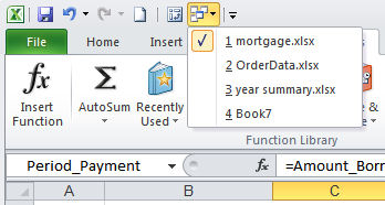
So, problem is… how can I switch between open documents in Excel or Word, for example, without having to use the Windows task bar? Solution is to use the Switch Windows button. I add it to the QAT (Quick Access Toolbar) and it totally makes sense to me.
In Excel or Word, click the Customize Quick Access Toolbar button and choose More Commands. From the list which currently shows Popular Commands choose All Commands and scroll to find the Switch Windows button and click Add.
Now it is on the QAT and it will show you all your open files and you can use it to switch between them by just clicking on the one to go to. Repeat the process for both Excel and Word and you’ll be happy – at least until something else bugs you!
Helen Bradley
Labels: Excel 2007, Excel 2010, filenames on task bar, Switch between open documents, switch between open worksheets, Windows 7, Word 2007, Word 2010, workbooks
Categories:Uncategorized
posted by Helen Bradley @ 8:58 am3 Comments links to this post
Monday, October 3rd, 2011

Consider this scenario – you have a cell which contains a link to data in another cell on another sheet. The link might be the only thing in the cell or it might be a link in a formula which contains references to data in lots of other cells too.
If you want to go to a particular referenced cell you could read off the cell details – its sheet name and its cell reference and navigate there yourself or you could get smart and have Excel do the work.
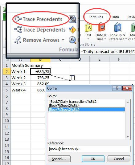
To do this, click in the cell containing the reference and choose Formulas > Trace Precedents. When you do this you will see a small sheet icon and an arrow with a black arrow head pointing at the cell. Hold your mouse cursor over the arrow until the mouse cursor turns into a hollow white arrow. Double click and the Go To dialog will open. In it will be references to all the cells in the formula. Click the reference you are interested in going to and the cell reference will be highlighted – click Ok and Excel will take you direct to that cell.
If you have both workbooks open the same process will work to take you to a cell in another workbook if it is referred to in a formula in the current workbook.
Helen Bradley
Labels: Excel 2007, Excel 2010, go to a cell, go to a cell on another sheet, go to a cell on another workbook, trace precedents
Categories:Uncategorized
posted by Helen Bradley @ 9:45 am1 Comment links to this post
Tuesday, September 20th, 2011

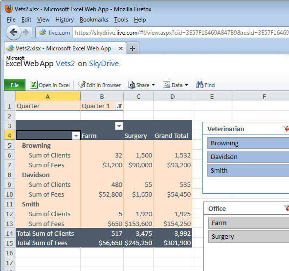
If you have access to a PC and an internet connection then your options for working with an Excel spreadsheet away from your desk are good – thanks to the Microsoft Office WebApps. Even though many of the advanced Excel tools you are used to using offline won’t be accessible online they won’t be destroyed by opening a file in the Excel WebApp either. You can view charts and filtered table data and features such as the new Slicers in an Excel 2010 PivotTable can be used to work with the data.
Of all the cloud based apps, including Google Docs, the Microsoft WebApps are your best option for working with Excel spreadsheets in the cloud when you are away from your desk and the apps are free.
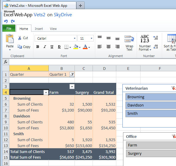
You can sign up for a free SkyDrive account at skydrive.live.com and that’s where you get access to the WebApps which include Excel, Word, PowerPoint and OneNote. I selected to upload this file then view it in the Excel viewer. To work on it beyond selecting options in the Slicers I can click Edit in Browser to open the file in the free cut down version of Excel online.

One benefit to using SkyDrive is that you can upload files from your local computer to SkyDrive where they are stored for you. You can work on the files online and later download them to your computer when you want to work on them there.
Helen Bradley
Labels: cloud Excel, Editing Excel files online, Excel 2010, Excel viewer, Excel WebApps, free Excel
Categories:Uncategorized
posted by Helen Bradley @ 4:50 pm1 Comment links to this post
Wednesday, June 29th, 2011

Much of the illustration Clip Art in the Microsoft Clip Organizer can be edited by changing its colors. By doing this you can not only recolor the art to match the look of your document but, if you use Theme colors then the art will change color when the Theme or Color scheme changes.
Now you won’t need information technology degrees to learn this – but maybe you’ll be so good at it, you just might consider graphic design college.
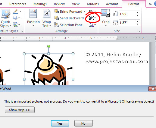
So, let’s see how the recoloring is done. First select the Clip Art and from the Picture Tools -> Format tab click the Group > Ungroup button. Answer Yes if you are prompted to convert the image to a Microsoft Office Drawing Object. In some applications such as Publisher you’ll need to repeat the process and select Ungroup again.

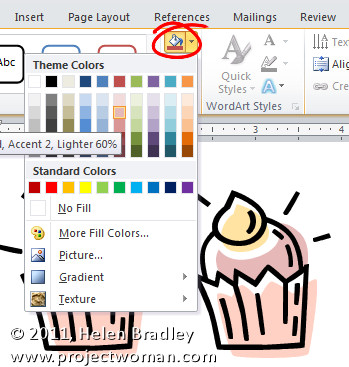
Now click on individual parts of the object and either remove them or recolor them by selecting a Shape Fill Color from the Drawing Tools > Format tab. If you use Theme colors then the colors will change later on when the theme changes.

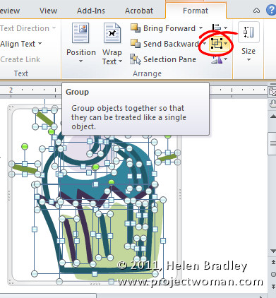
When you are done and you have recolored all the pieces you want to recolor, select all the pieces, right click and choose Group.

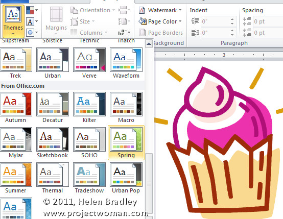
Change the document theme or Color Scheme to see the image change color to match the look of the theme.

Helen Bradley
Labels: clip art, color scheme, Excel 2010, Microsoft Office, Publisher 2010, recolor, theme, Word 2010
Categories:Uncategorized
posted by Helen Bradley @ 6:22 pm1 Comment links to this post
Tuesday, June 14th, 2011

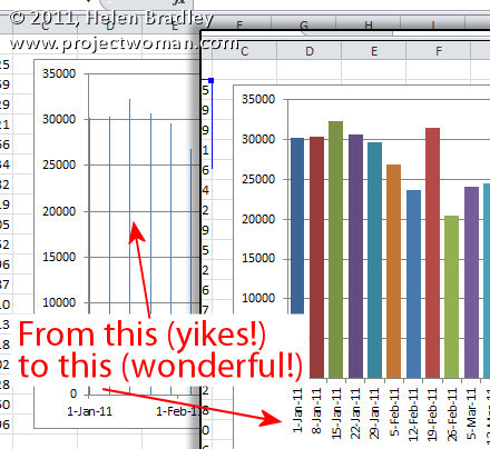
It’s probably happened to you, you’ve created an Excel chart and the columns are so narrow they are almost unreadable. The chart is ugly and it appears as if there’s nothing that you can do because nothing that should work does work.
The problem typically happens when you have a chart with an X axis that is has date data and where you aren’t plotting every day but, instead, for example, one day a week.
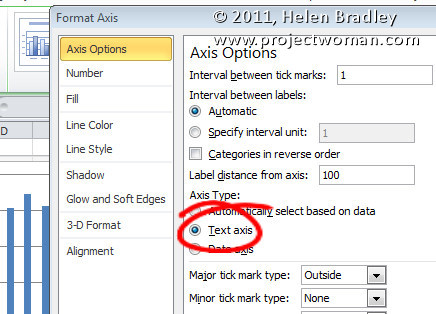
The solution is to click the X axis of the chart so that you have it selected, right click and choose Format Axis. From the Axis Options panel, select Text Axis. This turns your skinny bars into something a lot more attractive.

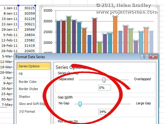
If the bars still not thick enough – and typically, for me, they aren’t – click on one bar to select the series, right click and choose Format Data Series. From the Series options, decrease the Gap Width value to around 35 percent. This option won’t work unless you first set the X axis to a Text axis although you and I both wish it would!

Helen Bradley
Labels: chart, column width, date axis, Excel 2010, gap
Categories:Uncategorized
posted by Helen Bradley @ 8:50 am86 Comments links to this post
Friday, June 10th, 2011

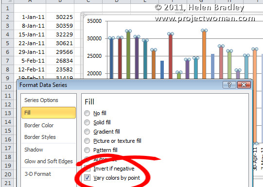
When you have a great big Excel column chart with heaps of delicious data but all in one series, it makes sense for the chart to be plotted in wonderful technicolor. However that’s an option Excel 2010 doesn’t make it very easy to find. If you try the Chart Tools > Design tab you can choose a multi-color chart but that only colors each series a different color so it won’t work when all your data is in one series.
The solution is to click on one column to select it then right click and choose Format Data Series > Fill group. Locate and check the Vary Colors by Point option and you’ll have a wonderful multi-colored series – much more enlightening than a plain old single color chart don’t you think?
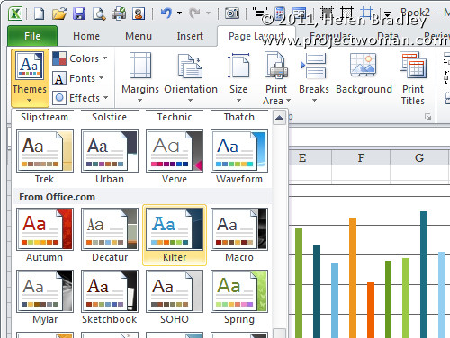
If the colors aren’t to your liking (you are getting just a little bit fussy but I do know exactly what you mean) select the Page Layout tab and check out the Themes – there’s sure to be one which will make your chart perfect.

Helen Bradley
Labels: chart, columns, Excel 2010, multi-color, themes
Categories:Uncategorized
posted by Helen Bradley @ 8:40 am20 Comments links to this post
Sunday, June 5th, 2011
 Some things Microsoft does make no sense at all. For this read showing the Developer Tab in Excel 2010. Ok first of all why hide the damn thing. Second of all why change how it is displayed from Excel 2007 to 2010 – yep they did – and yep it makes NO sense to do so.
The Developer tab contains some sweet goodies like form tools which let you put a button on a worksheet to run a macro – but you won’t know you can do this till you show the Developer tab.
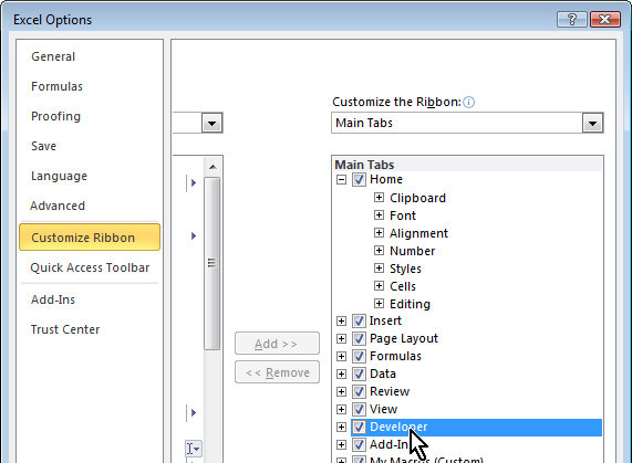
Ok… here’s how: Click the File button and click Customize Ribbon. In the left panel is the Developer toolbar but its checkbox is deselected. Click to check it and Voila! you now have a Developer tab.
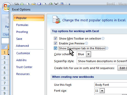
In Excel 2007, skip; the fuss – there is no Customize option and the option to display the Developer toolbar is in the first panel you see in the Excel Options dialog.

Helen Bradley
Labels: Developer toolbar, Excel 2007, Excel 2010
Categories:Uncategorized
posted by Helen Bradley @ 7:54 pm3 Comments links to this post
Friday, April 29th, 2011

In Excel 2003 and earlier you might recall that you could click a cell and choose Edit > Clear and choose to clear its Contents, Comments, Formatting or choose All to remove everything.
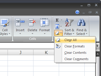
In Excel 2007/2010 there is a Clear Contents option on the right click menu but, in the absence of the Edit menu you’ll need to look elsewhere for the other options. On the Home tab of the Ribbon look for the Clear icon – it has an eraser on it and it has a dropdown list from which you can select the desired option.
It’s pretty obvious if you’re using Excel at full screen size but shrunk down it isn’t clear (pun intended) that it is there or what it does. I like to add the Clear All option to the Quick Access Toolbar so it’s easy to find and use. You will find it in the All Commands list and it is called Clear All if you’re looking for it.
Helen Bradley
Labels: delete cell contents, Excel 2007, Excel 2010
Categories:Uncategorized
posted by Helen Bradley @ 9:05 amNo Comments links to this post
Thursday, March 17th, 2011

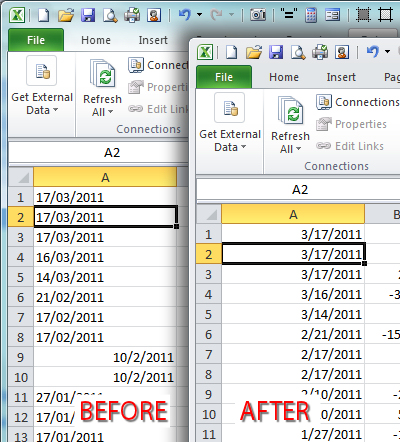
Today I encountered a problem when downloading some data from an Australian bank. Australia uses the DMY date format whereas the US uses MDY, my computer is set to use US as its region which means Excel expects dates to be entered using MDY format. Excel gets its country information which affects dates, in particular, from the setting you have for your Windows Region.
So, I had a .csv file in which all the dates were entered wrongly – they read 22/11/2010 instead of 11/22/2010, for example. When the dates are typed incorrectly for the country you are currently set to use, you can’t simply apply a format to them to fix the problem because there is no such date as 22/11/2010. And worse still a date like 2/1/2011 which is 2-Jan-2011 in Australia will be formatted as 1-Feb-2011 in my US Excel – throwing all my data spectacularly out.
So what to do?
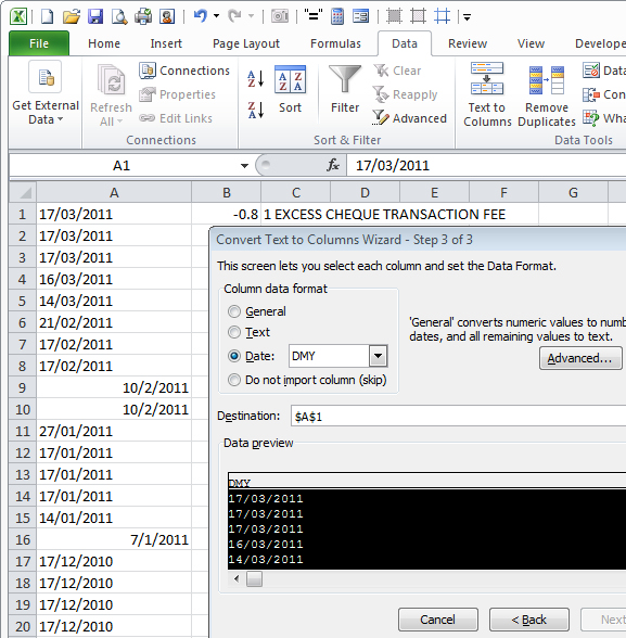
The simplest solution is to use the Excel data parse tool. Select the column of dates and choose Data > Text To Columns. This opens the Convert Text To Columns Wizard which is the old way of parsing data into Excel.
In Step 1 select either option as you only have one column of data selected anyway. Click Next twice. Now in step three of the wizard, select the Date option and select the formatting for the displayed data. So if the data has been typed in DMY format, select DMY. If it has been typed in MDY format, choose MDY. Click Finish.

The date data will be automatically converted to match the correct date syntax for your version of Excel. In short this converts all my Australian dates to US date format so they are correct in Excel. Select the column of dates and you can now format the dates using your preferred format.
It’s a simple but effective solution that avoids the necessity of retyping the date data.
Helen Bradley
Labels: convert, data, Dates, DMY, Excel, Excel 2010, MDY, parse
Categories:Uncategorized
posted by Helen Bradley @ 10:57 am30 Comments links to this post
Wednesday, June 16th, 2010
 If you are having difficulty understanding how a formula is calculating in Excel – perhaps because it appears to give you the wrong results – you can step through it to see how it is working.
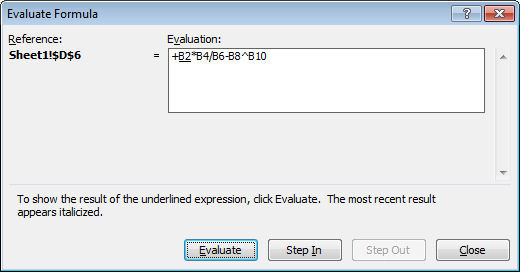
To do this, select the cell containing the formula and choose Tools > Formula Auditing > Evaluate Formula – in Excel 2007 find the Evaluate Formula option on the Formulas tab.
Click Evaluate and each time you do this, a portion of the formula will be evaluated and you can see it at work.
Use the Step In and Step Out options to see the actual values in place of any appropriate cell references.
This step by step processing should show you what is happening in your formula allowing you to troubleshoot any difficulties with it.
Helen Bradley
Labels: Excel 2003, Excel 2007, Excel 2010, Excel formulas, formula auditing, troubleshoot
Categories:Uncategorized
posted by Helen Bradley @ 7:04 am4 Comments links to this post


