

Monday, September 30th, 2013
Automatic Table of Contents in Google Docs

When creating a long document with many different sections, it’s often necessary to create a table of contents to make navigation easy. Fortunately, Google Docs can generate a table for you almost entirely automatically.
To do this, you must first create section headers using the list under Format > Paragraph Styles. Simply highlight a section title and apply an appropriate heading style for it. Each style grows progressively smaller from 1 to 6. Major sections, such as chapters, should use the largest headings while smaller subsections should use progressively smaller headings.
Once you have created all of your headings, select where you want the table of contents to be in your document and choose Insert > Table of Contents. The table will automatically fill with links to each heading and arrange itself according to the heading styles chosen. Smaller headings will be indented beneath larger headings in the table, indicating that they are subsections.
Labels: automatic, google docs, organize, table of contents
Friday, September 27th, 2013
Put the Apps back on my Chrome New Tab! NOW!

If the new Chrome Update (Sep 2013) messed up your browser, here’s how to get the old look back
Ok, I am rightly angry – my Chrome browser just updated and all the Apps on the New Tab (that I had laboriously configured and which I use daily because, hello Google I need them)disappeared.
Sure, I can click the new little Apps button on the Bookmark bar to view them – I get that – but why? I had Chrome all nice and organized – I didn’t need Google’s input to fix it… just like I don’t expect Google to walk into my house and rearrange my desk or my bookshelf or anything else I have organized the way I want it.
So, rant aside, here’s the solution to how to put the Chrome Apps back on the New Tab:
UPDATE:
As of Chrome 33 the option to fix the problem as detailed below (in red) has been removed. Seriously at Google people actually worked hard to remove this feature so we can no longer make Chrome behave the way we want it to? Way to go! Yet another reason I hate the Cloud and I hate apps that automatically update and companies that couldn’t care less about the needs of their user base. I just don’t understand why Google doesn’t listen to its users and help them out instead of giving us a totally useless Google search box in the middle of the new tab window. Now I understand that not everyone wants or likes the old style interface but why break the fix (that worked), for those of us who do?
Ok, today’s solution (until Google folk mess with this and break it too) is to download the New Tab Redirect app from the Chrome Web store here. Once installed, the Extension launches so you can set it to show your apps. So, you need the My New Tab page should show this URL to read:
chrome://apps
You can do this by typing the entry yourself or you can click the Apps button below Quick Save and it will be done automatically for you.

Now, in future when you click the New Tab button it will show your apps.
It works, no thanks to Google.
I hope this solution saves you from the stress of having Chrome apps disappear from your New Tab Page. It has certainly reduced my blood pressure!
1. Go to the address bar and type this in:
chrome://flags/
2. Press Enter and then search for this word:
Extended API
This will take you to the Extended API option which is set to Default
3. From the drop down list choose Disabled and then close and reopen Chrome.
Voila! your browser is now restored to its former glory!

Labels: apps button, changes, chrome apps on new tab, chrome browser updated, disappeared, fix, Google chrome, messed with, missing, restore, Undo
Wednesday, August 28th, 2013
Word 2013 Find only photos or illustrations

Learn how to find only photos or only illustrations when searching Office 2013 online images
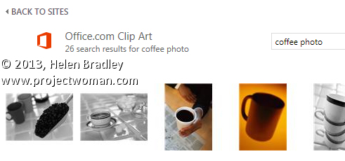
In Office 2013 the old Clip Art feature was removed and now you can insert an image by searching for it online at a number of places. One of these is the Microsoft clip art collection which is now stored totally online and not partly on your computer.
So far, so good.
The problem is that the old task pane feature which let you determine the types of images you want to search for is now gone. So, on the face of it, when you search for something like coffee you get illustrations and photos. In many cases much more than you want or need.
Often, I know ahead of time I want a photo or an illustration so I want my search to return only one type of image. There’s no information at all as to how to do this but you can! Instead of searching for coffee, type coffee photo to find photos relating to coffee or coffee wmf to find just illustrations as these are generally wmf format images.

It isn’t a perfect solution and you will miss out on some images as well as get the occasional illustration with your photos or vice versa.
However, if you’re not too fussy about missing out on some imagery then using this search format will weed out a lot of the stuff you don’t want and serve up mostly the type of content that you do want.
This tip works in any of the Office 2013 applications – PowerPoint 2013, Excel 2013, Publisher 2013. Word 2013 and more.
Labels: Excel 2013, filter, find photos, illustrations, PowerPoint 2013, Publisher 2013, search online images, wmf, Word 2013
Friday, August 23rd, 2013
Word 2010 and 2013 Tip – Markup the changes to your document

Keep track of the changes made to your document
Word’s Reviewing tools make it easy to show someone the changes you’ve made to a document.
You can set Word to record the changes before you make them by selecting the Review tab on the ribbon and click Track Changes > Track Changes.

Now, in Word 2007 & 2010, every addition to your document will be underlined and every deletion will be marked with strikeout. Word 2013 defaults to Simple Markup so you will need to choose All Markup to see the changes marked up.

These changes are retained when you save the document.
You can apply the changes permanently at any time by selecting Review > Accept or Reject and choose Accept All Changes (or Reject All Changes).

Word 2013 has a new feature which lets you force Track Changes to be enabled. Choose Review > Track Changes > Lock Tracking to enable this feature. Now if you save the document and send it to someone, any changes they make to the document will be recorded in the document. They cannot disable this feature without having the password to unlock the setting and disable it.
Labels: 2010, 2013, Accept All Changes, change, Highlight, Lock Tracking, mark, mark up, markup, Microsoft Office, Microsoft Word, review, tip, track changes, tracked changes, trick, Tutorial, up, Word, Word 2010, Word 2013
Thursday, August 15th, 2013
Word 2010 and 2013 Tip – How to sort data in a Word document

Sorting data in Word 2007, 2010 & 2013
In the pre-ribbon versions of Word you would use the Table commands to sort data in a Word document.
In Word 2007, 2010 & 2013 you can’t use the table sort options any longer for plain old text simply because you can’t select the table options if you don’t have a table – it’s a Catch 22 situation.
Luckily, Word now includes a proper sort option for any text – not just table text. To use it, first select the text to sort and then click the Sort button on the Home tab of the Ribbon.

When the Sort Text dialog opens you can choose what to sort such as Paragraph or Field and the type of sort. If you want a case sensitive sort so A is treated differently to a then click Options and check the Case Sensitive checkbox.

Once you are done select the sorting options, click Ok to perform the sort.
Labels: 07, 2007, 2010, 2013, Command, data, Microsoft Office, Microsoft Word, sort, Sort Options, Sort Text, table, Table Command, text, tip, trick, Tutorial, Word, Word 2010, Word 2013
Friday, August 9th, 2013
Word 2010 and 2013 Tip – Flow text through a document with linked text boxes

How to use linked text boxes to flow text throughout a document automatically
If you’re familiar with using desktop publishing software you’ll know that it is useful to be able to create text boxes and have the text flow automatically from one to the next. You use this feature to start a story on one page of a newsletter, for example, and to have it continue on a later page.
Word 2007, 2010 and 2013 can do this for you too, if you use the built in text box feature. To do this, first choose Insert > Text Box > Draw Text Box and click and drag to draw a text box on the page.

Repeat this and add a second text box on another page in the document.
Now select the first text box, right click and choose Create Text Box Link.

Now click in the second text box to link the two together.

In future, any text which you type into or paste into the first text box and which won’t fit because the box is not large enough to accommodate it, will flow automatically into the second text box.
Labels: 2010, 2013, automatic, Create Text Box Link, Draw Text Box, flow, insert, Microsoft Office, Microsoft Word, text, text box, tip, trick, Tutorial, Word, Word 2010, Word 2013
Thursday, August 1st, 2013
Word 2010 and 2013 Tip – Add a time and date stamp to a printed page

Know when your document was printed by adding a date and time stamp to each printed page
Add a date and time stamp all your printouts by placing the current date and time in the document footer so it prints when the page is printed.
To do this in Word 2007, 2010 and 2013 choose Insert > Footer > Edit Footer. Click the Date & Time button and enable the Update Automatically checkbox. From the list of dates and times choose a date or date and time – depending on what you want to see on the page. Click Ok.

Select the text that Word has inserted in the footer and you can now format it to a small font – such as Italic 8 pt. You can also prefix the text with the words Printed On: or something similar, if desired.

Click Close Header and Footer to return to your document. Now the current date and time will be printed in the footer each time the document is printed.
Labels: 2010, 2013, add, Close Header and Footer, date, footer, header, insert, Microsoft Office, Microsoft Word, Printed On, printout, stamp, time, timestamp, tip, trick, Tutorial, Update Automatically, Word, Word 2010, Word 2013
Tuesday, July 30th, 2013
Create a one click animation in PowerPoint 2013
Learn how to create a simple animation in PowerPoint. You will add a shape which, when clicked will trigger an image to be displayed. It is a smart animation with lots of potential uses which, once you see how it is done, will be simple to adapt to your own needs.
Transcript:
Hello, I’m Helen Bradley.
Welcome to this video tutorial. In this tutorial I’m going to show you how you can create an animation where you click a button to show an image. Before we get started with this tutorial let’s have a look and see what it is that we’re going to achieve.
I have an image here and a shape and when we play the presentation this is what we’re going to see. We’re going to see a slide without the picture and when I click on this shape I’ll see the image displayed. And we’re going to create this animation where we click on a shape and an image appears.
So back in PowerPoint let’s go to a new slide and I’ve already inserted my image. I just chose Insert and then Online Pictures. I searched for an elephant and I’ve just inserted it on the slide. So there’s nothing special about what I’ve done to date. Now I’m going to choose Insert and then Shapes and I’m going to choose my rounded rectangle shape.
And I’m going to add it to my slide and I’m going to add some text to it. And I’m just going to click away from the shape. Now that we have our shape and our image we’re ready to create the animation. To do this I’m going to click the Animations tab on the Ribbon. And I want to animate the elephant so I’m going to click on the elephant image and I’m going to choose an animation for it.
So I could choose an animation such as fade so it will fade in. And then I’m going to open the Animation task pane over here by clicking on Animation Pane because I want the elephant to be animated but I don’t want him to appear on a click and I don’t want him to appear after the slide is opened. I want him to appear when you click this particular shape.
And that’s a different animation. This is the elephant animation so I’m going to right click it and choose Effect Options because that allows me to control how this effect is going to play. And I’m going to click the Timing tab.
And I want this to be triggered by the clicking of this shape so I’m selecting to Start Effect on Click of and I’m going to select Rounded Rectangle and just click Ok. And now this image is going to animate when we click this shape. Let’s close down the task pane and let’s go and test it.
I’ll click the Slide Show. You have to do that because you have to test this slide as it would appear inside a working slide show. And you can see here we have our slide on the screen and just our filled rectangle. I’m gray. I have a trunk. Click to see what I am. The elephant image is not visible yet. However when I click the shape the elephant appears and we would then progress through the slide show.
So this is a simple animation effect that you can create so that you can click a shape and something happens. The animation is all added. All the effects are added to the image itself. You’re going to animate it with some sort of an entrance effect and then adjust its timing so that it is triggered by a click on this shape here.
I’m Helen Bradley.
Thank you for joining me for this video tutorial. Look out for more PowerPoint tutorials on this YouTube channel as well as additional tutorials on other Office applications and Photoshop, Lightroom and Illustrator.
Visit my website at helenbradley.com for tips, tricks and tutorials on all these applications.
Labels: animate, animate an image, animation taskpane, click to show an image, PowerPoint 2013, quiz, shape trigger, simple animation, test, trigger
Thursday, July 25th, 2013
Word 2010 and 2013 Tip – Making shapely images

Crop your image to a shape in Word
It is easy to crop an image to a shape such as a star or a heart in Word by using the Crop to Shape feature.
First add the image to your document then click to select it. From the Picture Tools > Format tab click Crop > Crop to Shape.

Select the shape to use to crop the image to. You can then add a shadow or reflection or other effect to the shape as desired.
Labels: 2010, 2013, AutoShape, crop, format, heart, image, Microsoft Office, Microsoft Word, Picture Tools, reflection, shadow, shape, star, thought bubble, tip, trick, Tutorial, Word, Word 2010, Word 2013
Monday, July 22nd, 2013
Create your first macro in Excel 2013
Learn how to type a macro in Excel 2007/2010 & 2013. Covers displaying the Developer tab and how to create your Personal Macro Workbook so you can create and save macros. Then how to create a new macro, save and run it.
Transcript:
Hello, I’m Helen Bradley. Welcome to this video tutorial. In this tutorial I’m going to show you how you can create a macro in the Visual Basic Editor in Microsoft Excel. First of all you need to make sure that this Developer tab is visible and it’s not by default. So this is Excel 2007. To make it visible you’ll click the Office button here, choose Excel Options and this is the option you want to enable Show Developer Tab in the Ribbon. With that selected the Developer tab then appears in the Ribbon. Now that’s only for Excel 2007. I’m actually going to close Excel 2007 because I’m going to work in 2010, but I just wanted to show you how you could get the Developer tab in 2007.
Now in 2010 and 2013 it’s a bit different. To get the Developer tab there you’ll choose File and then Options. And what you’re going to do is go to Customize Ribbon because only in 2010 and 2013 can you actually customize the Ribbon. And there’s an option here for Developer. So this the Developer tab and again by default it’s disabled so you want to just select it so that it is enabled and click Ok. Now this entire video was prompted by a user who asked me for a macro that would delete every row in a worksheet if there was nothing in column A.
So I have a worksheet here and I have some rows in which there is nothing at all and what we want to do is to delete them. So the first thing we need to do is to make sure that the Developer tab is visible on the Ribbon and then we’re going to actually create this macro. In fact I’m just going to copy and paste it because I just want to show you the basics of creating a macro. This might be one that you’ve been sent or it might be one you find on the web or whatever.
Now before you can actually create a macro inside the place where it’s supposed to be you have to actually have this one file created. And chances are if you’ve never created a macro before you don’t have the very file that you need. The simplest way to resolve that situation is to first before you do anything else go and click Record Macro. And you’re going to store this macro in what is called the personal macro workbook.
If you don’t have it Microsoft Excel creates it for you so that’s why we’re going to the trouble of recording just anything so that we can get this personal macro workbook created. And once it’s created then in future we’ll be able to store macros in it and these macros will always be available to every single worksheet.
Whenever Excel is opened it opens this file and everything is fine and dandy so I’m just going to click Ok. And I’m just going to type a couple of letters in there, press Enter. That’s a macro. That’s all it does and click Stop Recording. I don’t actually want the macro and I don’t actually want the contents of that cell. All I want is this special file that is called personal.xls. So I’m going to click Macros now and you can see here is the macro that we just created in this workbook personal.xls.
It’s personal.xlsb whatever it is for your particular version of Excel. And this is a file that Excel takes care of opening every time you come and open Excel so these macros are always going to be available. Now I want to add a new macro. And the macro I want to add is called remove rows. That’s just what I called it. So I’m going to type the word removerows. Now macro names have to be one whole word. You can’t use spaces but you can use underscores. I’m just going to type removerows.
And now because I don’t have that macro Excel is offering me the option of creating it. But I want to create this in my personal.xlsb workbook so I want to make sure that I select that first. Macro name personal.xlsb workbook, click Create. And what that does is it automatically opens the Visual Basic Editor for me so I don’t have to do all the work. And it also places me right in the middle of this code area which is exactly where I put my macro code. So I have it in a file so I’m just going to copy and paste it. In fact I’m going to do a little bit of the wrong thing so I can show you the result.
I’ve gone and got my file and I’ve copied the macro code to the clipboard and I’m going to paste it in. And you can see that what I did was I bought in the sub and end sub statements. And you can’t have two sets of sub and end sub statements. So the first thing I’m going to do is get rid of the extra statements. And it appears here that my lines have been cut in pieces so I’m just going to make sure that these comments are back in single lines.
So here is my removerows macro. And this has also got cut in two so let’s just neaten things up a little bit. And this is a macro that removes rows in a worksheet where the cell in column is blank. It doesn’t require you to make a selection before running it. However as Undo doesn’t work after running this macro it’s a good idea to back up your worksheet first. Well, that’s good. And I’m just going to while I’m here clean up this macro that I recorded earlier that I didn’t really want to keep but I just created so that I would get this personal.xlsb workbook.
Now that I’ve finished inside the Visual Basic Editor, I’ve created my macro I’m just going to choose File, Close and return to Microsoft Excel. Now the macro is stored not in this particular file but in this special workbook. I want to test it so the first thing I’ll do is to save my file just in case everything goes haywire. The other thing I’m going to do is just for my own purposes is format these particular rows the ones that I want to get rid of with a color. What I want to do is when I get rid of these rows the very first time I run it I just want to make sure that the macro is behaving correctly.
So if it were to do something funny I’ve marked up in orange exactly what I don’t want to see at the end of this macro. So if it were to do something like this, so let’s just go and do Delete Cells, I don’t want it to delete cells. I want it to delete a whole row so if it were to end up with something like this happening I know that my macro isn’t working. So I’m just setting myself up to check to make sure that everything is working correctly when I do run my macro. And if it works perfectly on this worksheet then I’m just going to assume that it’s going to work perfectly every other time in future.
So here we have our worksheet. Now it’s time to run the macro. Now you don’t have to use the Developer tab to do it although you can. But you can use the View tab. We’re going to Macros and here are our macros and the macros are in personal.xlsb. And the one we want to run is called removerows so I’m just going to click to run it. All the orange highlighting is gone and everything that is left are just rows that have data in column A.
So that’s how you would create a macro yourself if you found it on the web or you downloaded it from somewhere or were given it in the Visual Basic Editor in Excel. Once the personal.xlsb workbook has been created the first time you don’t have to go through that record macro step. That’s only to create that file the very first time. From now on Excel is going to take care of that file. If you’re prompted to save it when you exit Excel, say yes because you do want to save all the data that you’ve created in it. I’m Helen Bradley. Thank you for joining me for this video tutorial. Look out for more of my tutorials on this YouTube channel and visit projectwoman.com for tips, tricks and tutorials on a whole range of Office programs.
Labels: Create macro, developer tab, Excel 2013, first macro, new macro, Personal Macro Workbook, Ribbon, run macro, type macro
Thursday, July 11th, 2013
Word 2010 and 2013 Tip – Preview and Save a web page document

See your document as a web page and keep it looking that way
To see how any of your Word 2010 and 2013 documents will look when they are saved as web pages, select the View tab on the Ribbon, then click Web Layout.
Now, to save a document as a web page, select File > Save As. In the Save As dialog, under click the Save as type: dropdown list and choose Web Page (*.htm;*.html).

Make sure to choose a location to save the document in, give it a name (it should have the .htm extension), and click Save.
Labels: .htm, .html, 2010, 2013, file, File name, Microsoft Office, Microsoft Word, preview, save, Save As, save as type, tip, trick, Tutorial, view, Web, Web Layout, web page, Word, Word 2010, Word 2013
Monday, July 8th, 2013
Recolor clip art in Microsoft Office 2013 and earlier
Learn to recolor clip art using theme colors so it is not only the color that you want it to be but it also matches the theme and it changes color when the theme changes.
This works with pretty much all versions of Office and all apps including Word 2013, PowerPoint 2013, Excel 2013, Publisher 2013 and older versions of Office including 2010, 2007, 2003 and earlier.
Transcript:
Hello, I’m Helen Bradley.
Welcome to this video tutorial. In this tutorial I’m going to show you how you can easily recolor clipart in Microsoft Office and how you can use theme colors so that your clipart changes when your theme changes.
Before we get started with this tutorial let’s have a look and see what it is that we are trying to achieve. This is the same piece of clipart and I just made a duplicate of that clipart image and I recolored it in the way that I’m going to show you how you can recolor your clipart. But let’s have a look and see the impact of the recoloring.
I’m going to choose the Colors tool here and watch as I arrow over all of these colors in turn. And you’ll see that the clipart image that I have recolored I have recolored this time with theme colors. And the beauty of this is that the clipart image is going to change colors in accordance with the theme that is in use.
The only thing that hasn’t been recolored is the black and the little yellow light in the candle. Everything else is a theme color and it’s going to change color using the new theme colors whenever the theme or the design of this PowerPoint presentation changes. So this is the concept that we’re going for here.
Now I have a slightly simpler image here. All I did to find these images was I chose Insert and then Online Pictures and I went looking for cake. And I particularly wanted wmf files as that’s Windows metafile and that is an illustrative file most of which can be recolored inside of PowerPoint or Word or Excel or any of the Microsoft applications.
And you don’t have to be using Microsoft Office 2013. You can choose any version of Microsoft Office. I’ve been doing this for years in Microsoft Office. It’s just that the way that you add images is a little bit different in this new version. Now before I start let’s just take a copy of this image and let’s paste it so that we’re working on a duplicate.
We can see then how far we’ve come later on. I’m just going to get rid of these images. Now with the image that I’m working on selected I’m going to choose Picture Tools, Format tab and I’m going to choose Group and then Ungroup.
Now you’ll see that the group option sometimes is not available from this dropdown menu but it will always be available from the Picture Tools, Format tab if the image is able to be ungrouped. You’ll get a message showing that this is an imported picture and not a group and asking you if you want to convert it to a Microsoft Office drawing object.
The answer to that is yes. And then you’ll go and repeat the process. You’ll right click and choose Group, Ungroup or from the Drawing Tools, Format tab you’ll choose the Group button here and choose Ungroup.
That ungroups the object so it’s now a whole lot of smaller objects. I’m just going to click outside it and then we’re going to start selecting individual pieces of this object. And I suggest that you start with a nice color scheme. So I’m just going to go to the color schemes and let’s choose something relatively colorful.
I found slip stream was a good option to use but any of these such as red violet that is fairly colorful is a good choice. Drawing Tools, Format tab and now from the shape filled dropdown list we’re going to make sure that we recolor all of the shapes using the fill colors that are theme colors.
So, again, I’m going to select here, this is on this sort of turquoise bit, and I’m going to color it a darker version of that same blue. I’m going to click on the candle light and see if I’ve got something I can use for candle light. I think I’m going to choose one of these colors because I would really like my candle light this time to be a theme color.
To select multiple colors or multiple shapes at a time I’m just selecting the first and then Ctrl clicking on the last. And again, I want these to be colored the same color as the candle light. Now I’m going to click here. There’s a shape here.
If you ever want to see what the shape is that you’re working on just press the Delete key and it will disappear and then you can undo it to be able to work on it. Or of course you can just fill it and see what it is that you are actually filling.
So I’m going to select that color. And now we’re going for this shape over here and I want a slightly darker or lighter version here. I think I’m going for a darker version. And here we have the shadows. Again, I’ll want a darker color for the shadow. I think I’ll go back for these blues. I’m going to stick to the turquoises and this sort of purple color.
So I’m going to now select these smaller items here and when I’ve got them selected I’m going to fill them as well. And when I’m pretty happy with my shape that has been recolored I’m going to select over the entire shape because now what I want to do is to stick it all back together again because I don’t want lots of little pieces.
Drawing Tools, Format tab, Group and this time I want to Regroup. And I’ll just test this by moving the object and it should all move as one. And now let’s look and see that this object is going to recolor unlike the original object if we change the color of this particular design that we’re using in PowerPoint.
So I’m going to choose the colors dropdown list here and as I choose a different color scheme you can see that my clipart shape is changing color. And as I said this works exactly the same way in any of the Office applications and in pretty near any version of these. You can do this in Word 2003.
You can do it in PowerPoint, Excel, Publisher, any of the applications and you can create clipart so that it not only matches the current theme but also looks the colors that you want it to look but which will change colors as the theme colors change.
I’m Helen Bradley.
Thank you for joining me for this video tutorial. Look out for more of my PowerPoint and Microsoft Office tutorials on this YouTube channel.
And visit my website at projectwoman.com for more tips, tricks and tutorials on a range of Microsoft Office applications as well as Photoshop, Lightroom, Illustrator and a whole lot more.
Labels: clip art, Clipart, edit clip art, Excel 2013, Microsoft Office 2013, Office 2003, Office 2007, Office 2010, PowerPoint 2013, Publisher 2013, recolor, recolour, theme, theme colors, wmf, Word 2013